使用 TensorFlow 2 和 Keras 在 Python 中使用 Long Short-Term Memory Recurrent Neural Network 预测不同的股票价格。
TensorFlow 2和Keras预测股票价格:预测股价一直是对投资者和研究人员都很有吸引力的话题。投资者总是质疑一只股票的价格会不会上涨,因为有很多复杂的财务指标只有投资者和有良好金融知识的人才能理解,股市的走势是不一致的,在普通人看来很随意。
机器学习是非专家能够准确预测并获得稳定财富的绝佳机会,并且可以帮助专家获得最有用的指标并做出更好的预测。
Python如何预测股票价格?本教程的目的是在TensorFlow 2和 Keras 中构建一个预测股市价格的神经网络。更具体地说,我们将使用LSTM 单元构建一个循环神经网络,因为它是当前时间序列预测中的最新技术。
好的,让我们开始吧。首先,你需要安装 Tensorflow 2 和其他一些库:
pip3 install tensorflow pandas numpy matplotlib yahoo_fin sklearn有关如何在此处安装 Tensorflow 2 的更多信息。
Python预测股票价格示例:完成所有设置后,打开一个新的 Python 文件(或笔记本)并导入以下库:
import tensorflow as tf
from tensorflow.keras.models import Sequential
from tensorflow.keras.layers import LSTM, Dense, Dropout, Bidirectional
from tensorflow.keras.callbacks import ModelCheckpoint, TensorBoard
from sklearn import preprocessing
from sklearn.model_selection import train_test_split
from yahoo_fin import stock_info as si
from collections import deque

import os
import numpy as np
import pandas as pd
import random我们使用的是yahoo_fin模块,它本质上是一个从 Yahoo Finance 平台提取财务数据的 Python 爬虫,所以它不是一个可靠的 API,请随意使用其他数据源,例如Alpha Vantage。
此外,我们需要确保在运行我们的训练/测试后我们得到稳定的结果,设置种子将有助于:
# set seed, so we can get the same results after rerunning several times
np.random.seed(314)
tf.random.set_seed(314)
random.seed(314)
还学习: 如何在 Python 中使用 Keras 构建垃圾邮件分类器。
准备数据集
作为第一步,我们需要编写一个函数,从 Internet 下载数据集并对其进行预处理:
def shuffle_in_unison(a, b):
    # shuffle two arrays in the same way
    state = np.random.get_state()
    np.random.shuffle(a)
    np.random.set_state(state)
    np.random.shuffle(b)

def load_data(ticker, n_steps=50, scale=True, shuffle=True, lookup_step=1, split_by_date=True,
                test_size=0.2, feature_columns=['adjclose', 'volume', 'open', 'high', 'low']):
    """
    Loads data from Yahoo Finance source, as well as scaling, shuffling, normalizing and splitting.
    Params:
        ticker (str/pd.DataFrame): the ticker you want to load, examples include AAPL, TESL, etc.
        n_steps (int): the historical sequence length (i.e window size) used to predict, default is 50
        scale (bool): whether to scale prices from 0 to 1, default is True
        shuffle (bool): whether to shuffle the dataset (both training & testing), default is True
        lookup_step (int): the future lookup step to predict, default is 1 (e.g next day)
        split_by_date (bool): whether we split the dataset into training/testing by date, setting it
            to False will split datasets in a random way
        test_size (float): ratio for test data, default is 0.2 (20% testing data)
        feature_columns (list): the list of features to use to feed into the model, default is everything grabbed from yahoo_fin
    """
    # see if ticker is already a loaded stock from yahoo finance
    if isinstance(ticker, str):
        # load it from yahoo_fin library
        df = si.get_data(ticker)
    elif isinstance(ticker, pd.DataFrame):
        # already loaded, use it directly
        df = ticker
    else:
        raise TypeError("ticker can be either a str or a `pd.DataFrame` instances")
    # this will contain all the elements we want to return from this function
    result = {}
    # we will also return the original dataframe itself
    result['df'] = df.copy()
    # make sure that the passed feature_columns exist in the dataframe
    for col in feature_columns:
        assert col in df.columns, f"'{col}' does not exist in the dataframe."
    # add date as a column
    if "date" not in df.columns:
        df["date"] = df.index
    if scale:
        column_scaler = {}
        # scale the data (prices) from 0 to 1
        for column in feature_columns:
            scaler = preprocessing.MinMaxScaler()
            df[column] = scaler.fit_transform(np.expand_dims(df[column].values, axis=1))
            column_scaler[column] = scaler
        # add the MinMaxScaler instances to the result returned
        result["column_scaler"] = column_scaler
    # add the target column (label) by shifting by `lookup_step`
    df['future'] = df['adjclose'].shift(-lookup_step)
    # last `lookup_step` columns contains NaN in future column
    # get them before droping NaNs
    last_sequence = np.array(df[feature_columns].tail(lookup_step))
    # drop NaNs
    df.dropna(inplace=True)
    sequence_data = []
    sequences = deque(maxlen=n_steps)
    for entry, target in zip(df[feature_columns + ["date"]].values, df['future'].values):
        sequences.append(entry)
        if len(sequences) == n_steps:
            sequence_data.append([np.array(sequences), target])
    # get the last sequence by appending the last `n_step` sequence with `lookup_step` sequence
    # for instance, if n_steps=50 and lookup_step=10, last_sequence should be of 60 (that is 50+10) length
    # this last_sequence will be used to predict future stock prices that are not available in the dataset
    last_sequence = list([s[:len(feature_columns)] for s in sequences]) + list(last_sequence)
    last_sequence = np.array(last_sequence).astype(np.float32)
    # add to result
    result['last_sequence'] = last_sequence
    # construct the X's and y's
    X, y = [], []
    for seq, target in sequence_data:
        X.append(seq)
        y.append(target)
    # convert to numpy arrays
    X = np.array(X)
    y = np.array(y)
    if split_by_date:
        # split the dataset into training & testing sets by date (not randomly splitting)
        train_samples = int((1 - test_size) * len(X))
        result["X_train"] = X[:train_samples]
        result["y_train"] = y[:train_samples]
        result["X_test"]  = X[train_samples:]
        result["y_test"]  = y[train_samples:]
        if shuffle:
            # shuffle the datasets for training (if shuffle parameter is set)
            shuffle_in_unison(result["X_train"], result["y_train"])
            shuffle_in_unison(result["X_test"], result["y_test"])
    else:
        # split the dataset randomly
        result["X_train"], result["X_test"], result["y_train"], result["y_test"] = train_test_split(X, y,
                                                                                test_size=test_size, shuffle=shuffle)
    # get the list of test set dates
    dates = result["X_test"][:, -1, -1]
    # retrieve test features from the original dataframe
    result["test_df"] = result["df"].loc[dates]
    # remove duplicated dates in the testing dataframe
    result["test_df"] = result["test_df"][~result["test_df"].index.duplicated(keep='first')]
    # remove dates from the training/testing sets & convert to float32
    result["X_train"] = result["X_train"][:, :, :len(feature_columns)].astype(np.float32)
    result["X_test"] = result["X_test"][:, :, :len(feature_columns)].astype(np.float32)
    return result
这个函数很长但很方便,它接受几个参数以尽可能灵活:
- 该
ticker参数是我们要加载的股票,例如,你可以使用TSLA为特斯拉股市,AAPL苹果,等等。它也可以是一个 Pandas Dataframe,条件是它包含列feature_columns以及日期作为索引。 n_steps整数表示我们要使用的历史序列长度,有人称之为窗口大小,回忆一下我们要使用一个循环神经网络,我们需要向网络中输入一个序列数据,选择50表示我们将使用50天的股票价格来预测下一个查找时间步长。scale是一个布尔变量,指示是否将价格从0缩放到1 ,我们将其设置True为将高值从0缩放到1将有助于神经网络更快、更有效地学习。lookup_step是要预测的未来查找步骤,默认设置为1(例如第二天)。15表示接下来的15天,以此类推。split_by_date是一个布尔值,表示我们是否按日期拆分训练和测试集,将其设置为False意味着我们使用sklearn的train_test_split()函数将数据随机拆分为训练和测试。如果是True(默认),我们按日期顺序拆分数据。
TensorFlow 2和Keras预测股票价格:我们将使用此数据集中的所有可用功能,即open、high、low、volume和调整后的 close。请查看本教程以了解有关这些指标的更多信息。
上述函数执行以下操作:
- 首先,它使用yahoo_fin模块中的stock_info.get_data()函数加载数据集。
"date"如果它不存在,它会添加索引中的列,这将有助于我们稍后获取测试集的功能。- 如果scale参数作为True传递,它将使用sklearn的MinMaxScaler类将所有价格从0缩放到1(包括volume)。请注意,每列都有自己的缩放器。
- 然后通过将调整后的关闭列移动lookup_step来添加表示目标值(要预测的标签或 y 的标签)的未来列。
- 之后,它将数据打乱并拆分为训练集和测试集,最后返回结果。
为了更好地理解代码,我强烈建议你手动打印输出变量 ( result ) 并查看功能和标签是如何制作的。
还学习: 如何使用 Python 和 Scikit-learn 制作语音情感识别器。
模型创建
Python预测股票价格示例 - 现在我们有一个合适的函数来加载和准备数据集,我们需要另一个核心函数来构建我们的模型:
def create_model(sequence_length, n_features, units=256, cell=LSTM, n_layers=2, dropout=0.3,
                loss="mean_absolute_error", optimizer="rmsprop", bidirectional=False):
    model = Sequential()
    for i in range(n_layers):
        if i == 0:
            # first layer
            if bidirectional:
                model.add(Bidirectional(cell(units, return_sequences=True), batch_input_shape=(None, sequence_length, n_features)))
            else:
                model.add(cell(units, return_sequences=True, batch_input_shape=(None, sequence_length, n_features)))
        elif i == n_layers - 1:
            # last layer
            if bidirectional:
                model.add(Bidirectional(cell(units, return_sequences=False)))
            else:
                model.add(cell(units, return_sequences=False))
        else:
            # hidden layers
            if bidirectional:
                model.add(Bidirectional(cell(units, return_sequences=True)))
            else:
                model.add(cell(units, return_sequences=True))
        # add dropout after each layer
        model.add(Dropout(dropout))
    model.add(Dense(1, activation="linear"))
    model.compile(loss=loss, metrics=["mean_absolute_error"], optimizer=optimizer)
return model同样,此功能也很灵活,你可以更改层数、辍学率、RNN单元、损失和用于编译模型的优化器。上面的函数构造了一个RNN,它有一个具有1 个神经元的密集层作为输出层,这个模型需要一个序列长度为序列的特征 序列(在这种情况下,我们将通过50或100 个)连续时间步长(在这个数据集中是天)并输出一个指示下一个时间步长的价格的值。
它也接受n_features作为参数,这是我们将通过对每个序列,在我们的例子了一些功能,我们会通过adjclose,open,high,low和volume 列(即5个功能)。
你可以根据需要调整默认参数,n_layers是要堆叠的 RNN 层数,dropout是每个 RNN 层后的丢失率,units是 RNNcell单元的数量(无论是LSTM、SimpleRNN还是GRU),bidirectional是指示是否使用双向 RNN 的布尔值,请尝试使用它们!
训练模型
Python如何预测股票价格?现在我们已准备好所有核心功能,让我们训练我们的模型,但在此之前,让我们初始化所有参数(以便你稍后可以根据需要对其进行编辑):
import os
import time
from tensorflow.keras.layers import LSTM

# Window size or the sequence length
N_STEPS = 50
# Lookup step, 1 is the next day
LOOKUP_STEP = 15
# whether to scale feature columns & output price as well
SCALE = True
scale_str = f"sc-{int(SCALE)}"
# whether to shuffle the dataset
SHUFFLE = True
shuffle_str = f"sh-{int(SHUFFLE)}"
# whether to split the training/testing set by date
SPLIT_BY_DATE = False
split_by_date_str = f"sbd-{int(SPLIT_BY_DATE)}"
# test ratio size, 0.2 is 20%
TEST_SIZE = 0.2
# features to use
FEATURE_COLUMNS = ["adjclose", "volume", "open", "high", "low"]
# date now
date_now = time.strftime("%Y-%m-%d")
### model parameters
N_LAYERS = 2
# LSTM cell
CELL = LSTM
# 256 LSTM neurons
UNITS = 256
# 40% dropout
DROPOUT = 0.4
# whether to use bidirectional RNNs
BIDIRECTIONAL = False
### training parameters
# mean absolute error loss
# LOSS = "mae"
# huber loss
LOSS = "huber_loss"
OPTIMIZER = "adam"
BATCH_SIZE = 64
EPOCHS = 500
# Amazon stock market
ticker = "AMZN"
ticker_data_filename = os.path.join("data", f"{ticker}_{date_now}.csv")
# model name to save, making it as unique as possible based on parameters
model_name = f"{date_now}_{ticker}-{shuffle_str}-{scale_str}-{split_by_date_str}-\
{LOSS}-{OPTIMIZER}-{CELL.__name__}-seq-{N_STEPS}-step-{LOOKUP_STEP}-layers-{N_LAYERS}-units-{UNITS}"
if BIDIRECTIONAL:
    model_name += "-b"
所以上面的代码是关于定义我们要使用的所有超参数,我们解释了其中的一些,而我们没有解释其他的:
TEST_SIZE:测试集率。例如总数据集的0.2平均值20%。FEATURE_COLUMNS:我们将用来预测下一个价格的特征。N_LAYERS:要使用的 RNN 层数。CELL:要使用的 RNN 单元,默认为 LSTM。UNITS:cell单位数。DROPOUT:dropout rate 是在一个层中没有训练给定节点的概率,其中 0.0 表示根本没有 dropout。这种类型的正则化可以帮助模型不过度拟合我们的训练数据。BIDIRECTIONAL:是否使用双向循环神经网络。LOSS:用于此回归问题的损失函数,我们使用Huber 损失,你也可以使用平均绝对误差 (mae) 或均方误差 (mse)。OPTIMIZER:要使用的优化算法,默认为Adam。BATCH_SIZE:每次训练迭代使用的数据样本数。EPOCHS:学习算法将通过整个训练数据集的次数,我们在这里使用了 500,但尝试进一步增加它。
随意尝试这些值以获得比我更好的结果。
Python预测股票价格示例:好的,让我们在训练之前确保results、logs和data文件夹存在:
# create these folders if they does not exist
if not os.path.isdir("results"):
    os.mkdir("results")
if not os.path.isdir("logs"):
    os.mkdir("logs")
if not os.path.isdir("data"):
    os.mkdir("data")
最后,让我们调用上述函数来训练我们的模型:
# load the data
data = load_data(ticker, N_STEPS, scale=SCALE, split_by_date=SPLIT_BY_DATE,
                shuffle=SHUFFLE, lookup_step=LOOKUP_STEP, test_size=TEST_SIZE,
                feature_columns=FEATURE_COLUMNS)
# save the dataframe
data["df"].to_csv(ticker_data_filename)
# construct the model
model = create_model(N_STEPS, len(FEATURE_COLUMNS), loss=LOSS, units=UNITS, cell=CELL, n_layers=N_LAYERS,
                    dropout=DROPOUT, optimizer=OPTIMIZER, bidirectional=BIDIRECTIONAL)
# some tensorflow callbacks
checkpointer = ModelCheckpoint(os.path.join("results", model_name + ".h5"), save_weights_only=True, save_best_only=True, verbose=1)
tensorboard = TensorBoard(log_dir=os.path.join("logs", model_name))
# train the model and save the weights whenever we see
# a new optimal model using ModelCheckpoint
history = model.fit(data["X_train"], data["y_train"],
                    batch_size=BATCH_SIZE,
                    epochs=EPOCHS,
                    validation_data=(data["X_test"], data["y_test"]),
                    callbacks=[checkpointer, tensorboard],
verbose=1)我们使用了ModelCheckpoint,它在训练期间的每个 epoch 中保存我们的模型。我们还使用TensorBoard来可视化训练过程中的模型性能。运行上述代码块后,它将训练模型 5 00 个epochs(如我们之前设置的),因此需要一些时间,这是第一行输出:
Train on 4696 samples, validate on 1175 samples
Epoch 1/500
4608/4696 [============================>.] - ETA: 0s - loss: 0.0011 - mean_absolute_error: 0.0211
Epoch 00001: val_loss improved from inf to 0.00011, saving model to results\2020-12-11_AMZN-sh-1-sc-1-sbd-0-huber_loss-adam-LSTM-seq-50-step-15-layers-2-units-256.h5
4696/4696 [==============================] - 7s 2ms/sample - loss: 0.0011 - mean_absolute_error: 0.0211 - val_loss: 1.0943e-04 - val_mean_absolute_error: 0.0071
Epoch 2/500
4544/4696 [============================>.] - ETA: 0s - loss: 4.3212e-04 - mean_absolute_error: 0.0146
Epoch 00002: val_loss did not improve from 0.00011
4696/4696 [==============================] - 2s 411us/sample - loss: 4.2579e-04 - mean_absolute_error: 0.0144 - val_loss: 1.5914e-04 - val_mean_absolute_error: 0.0104训练结束后(或训练期间),尝试tensorboard使用以下命令运行:
tensorboard --logdir="logs"现在这将在localhost:6006启动一个本地HTTP服务器,进入浏览器后,你会看到类似这样的内容:
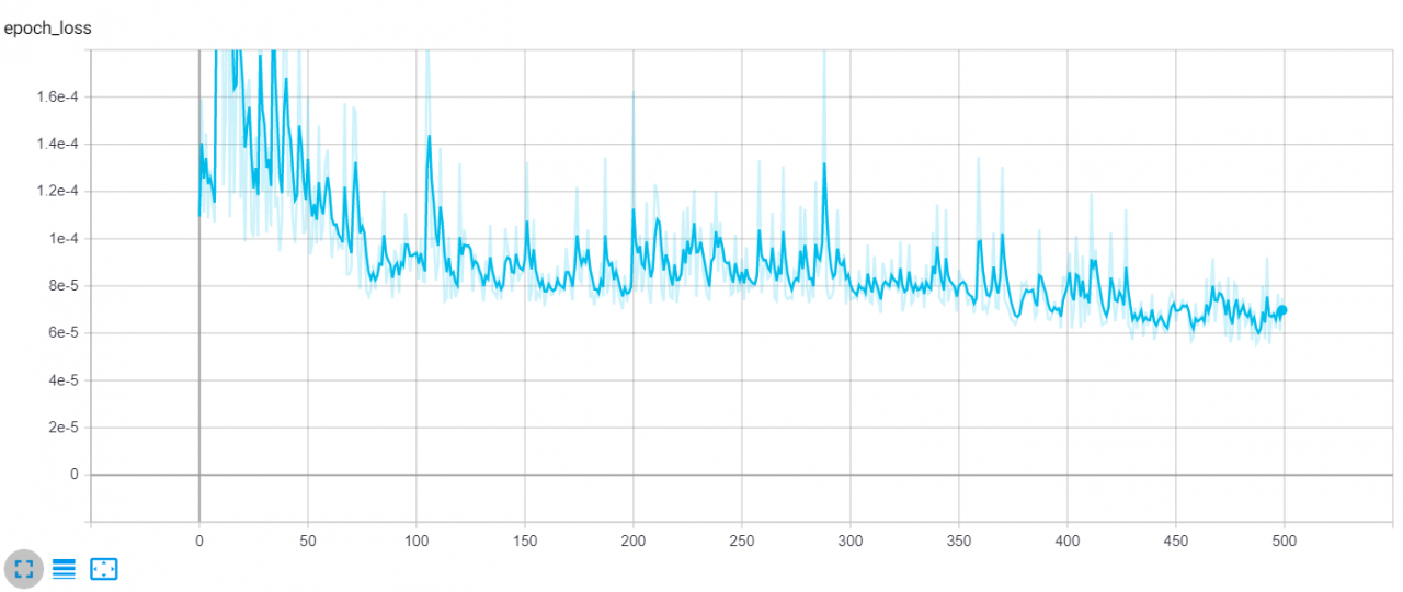
损失是参数中指定的Huber 损失LOSS(你可以随时将其更改为均值绝对误差或均方误差),曲线是验证损失。如你所见,它随着时间的推移显着减少,你还可以增加 epoch 数以获得更好的结果。
测试模型
TensorFlow 2和Keras预测股票价格:现在我们已经训练了我们的模型,让我们评估它并看看它在测试集上的表现如何,下面的函数采用一个 Pandas 数据框并使用matplotlib在同一图中绘制真实价格和预测价格,我们稍后将使用它:
import matplotlib.pyplot as plt

def plot_graph(test_df):
    """
    This function plots true close price along with predicted close price
    with blue and red colors respectively
    """
    plt.plot(test_df[f'true_adjclose_{LOOKUP_STEP}'], c='b')
    plt.plot(test_df[f'adjclose_{LOOKUP_STEP}'], c='r')
    plt.xlabel("Days")
    plt.ylabel("Price")
    plt.legend(["Actual Price", "Predicted Price"])
plt.show()Python如何预测股票价格?下面的函数将model与data该被返回create_model()和load_data()功能分别,并构造一个数据帧中,它包括与真正的未来adjclose,以及计算买入和卖出获利沿预计adjclose,我们会看到它在行动中片刻:
def get_final_df(model, data):
    """
    This function takes the `model` and `data` dict to
    construct a final dataframe that includes the features along
    with true and predicted prices of the testing dataset
    """
    # if predicted future price is higher than the current,
    # then calculate the true future price minus the current price, to get the buy profit
    buy_profit  = lambda current, pred_future, true_future: true_future - current if pred_future > current else 0
    # if the predicted future price is lower than the current price,
    # then subtract the true future price from the current price
    sell_profit = lambda current, pred_future, true_future: current - true_future if pred_future < current else 0
    X_test = data["X_test"]
    y_test = data["y_test"]
    # perform prediction and get prices
    y_pred = model.predict(X_test)
    if SCALE:
        y_test = np.squeeze(data["column_scaler"]["adjclose"].inverse_transform(np.expand_dims(y_test, axis=0)))
        y_pred = np.squeeze(data["column_scaler"]["adjclose"].inverse_transform(y_pred))
    test_df = data["test_df"]
    # add predicted future prices to the dataframe
    test_df[f"adjclose_{LOOKUP_STEP}"] = y_pred
    # add true future prices to the dataframe
    test_df[f"true_adjclose_{LOOKUP_STEP}"] = y_test
    # sort the dataframe by date
    test_df.sort_index(inplace=True)
    final_df = test_df
    # add the buy profit column
    final_df["buy_profit"] = list(map(buy_profit,
                                    final_df["adjclose"],
                                    final_df[f"adjclose_{LOOKUP_STEP}"],
                                    final_df[f"true_adjclose_{LOOKUP_STEP}"])
                                    # since we don't have profit for last sequence, add 0's
                                    )
    # add the sell profit column
    final_df["sell_profit"] = list(map(sell_profit,
                                    final_df["adjclose"],
                                    final_df[f"adjclose_{LOOKUP_STEP}"],
                                    final_df[f"true_adjclose_{LOOKUP_STEP}"])
                                    # since we don't have profit for last sequence, add 0's
                                    )
    return final_df
我们要定义的最后一个函数是负责预测下一个未来价格的函数:
def predict(model, data):
    # retrieve the last sequence from data
    last_sequence = data["last_sequence"][-N_STEPS:]
    # expand dimension
    last_sequence = np.expand_dims(last_sequence, axis=0)
    # get the prediction (scaled from 0 to 1)
    prediction = model.predict(last_sequence)
    # get the price (by inverting the scaling)
    if SCALE:
        predicted_price = data["column_scaler"]["adjclose"].inverse_transform(prediction)[0][0]
    else:
        predicted_price = prediction[0][0]
    return predicted_price
现在我们有了评估模型的必要函数,让我们加载最佳权重并继续评估:
# load optimal model weights from results folder
model_path = os.path.join("results", model_name) + ".h5"
model.load_weights(model_path)使用model.evaluate()方法计算损失和平均绝对误差:
# evaluate the model
loss, mae = model.evaluate(data["X_test"], data["y_test"], verbose=0)
# calculate the mean absolute error (inverse scaling)
if SCALE:
    mean_absolute_error = data["column_scaler"]["adjclose"].inverse_transform([[mae]])[0][0]
else:
mean_absolute_error = mae我们还考虑了缩放的输出值,因此如果参数设置为,我们将使用我们之前在函数中定义的inverse_transform()方法。MinMaxScalerload_data()SCALETrue
现在让我们调用get_final_df()我们之前定义的函数来构建我们的测试集数据框:
# get the final dataframe for the testing set
final_df = get_final_df(model, data)另外,让我们使用predict()函数来获取未来价格:
# predict the future price
future_price = predict(model, data)
Python如何预测股票价格?下面的代码通过计算正利润(买入利润和卖出利润)的数量来计算准确度分数:
# we calculate the accuracy by counting the number of positive profits
accuracy_score = (len(final_df[final_df['sell_profit'] > 0]) + len(final_df[final_df['buy_profit'] > 0])) / len(final_df)
# calculating total buy & sell profit
total_buy_profit  = final_df["buy_profit"].sum()
total_sell_profit = final_df["sell_profit"].sum()
# total profit by adding sell & buy together
total_profit = total_buy_profit + total_sell_profit
# dividing total profit by number of testing samples (number of trades)
profit_per_trade = total_profit / len(final_df)
我们还计算每笔交易的利润,这实质上是总利润除以测试样本的数量。打印所有先前计算的指标:
# printing metrics
print(f"Future price after {LOOKUP_STEP} days is {future_price:.2f}$")
print(f"{LOSS} loss:", loss)
print("Mean Absolute Error:", mean_absolute_error)
print("Accuracy score:", accuracy_score)
print("Total buy profit:", total_buy_profit)
print("Total sell profit:", total_sell_profit)
print("Total profit:", total_profit)
print("Profit per trade:", profit_per_trade)
输出:
Future price after 15 days is 3232.24$
huber_loss loss: 8.655239071231335e-05
Mean Absolute Error: 24.113272707281315
Accuracy score: 0.5884808013355592
Total buy profit: 10710.308540344238
Total sell profit: 2095.779877185823
Total profit: 12806.088417530062
Profit per trade: 10.68955627506683太好了,模型说15天后AMZN的价格会是3232.24$,这很有趣!
以下是主要指标的含义:
- 平均绝对误差:我们得到大约 20 的误差,这意味着,平均而言,模型预测与真实价格相差20 多美元,这会因价格而异
ticker,随着价格变大,误差也会增加。因此,你应该仅在股票代码稳定时(例如AMZN)使用此指标来比较你的模型。 - 买入/卖出利润:这是我们在所有测试样本上开仓时获得的利润,我们根据
get_final_df()函数计算了这些利润。 - 总利润:这只是买入和卖出利润的总和。
- 每笔交易利润:总利润除以测试样本总数。
- 准确度分数:这是我们预测准确度的分数,此计算基于我们从测试样本的所有交易中获得的正利润。
我邀请你调整参数或更改参数LOOKUP_STEP以获得最佳可能的误差、准确性和利润!
现在让我们绘制显示实际价格和预测价格的图表:
# plot true/pred prices graph
plot_graph(final_df)
结果:
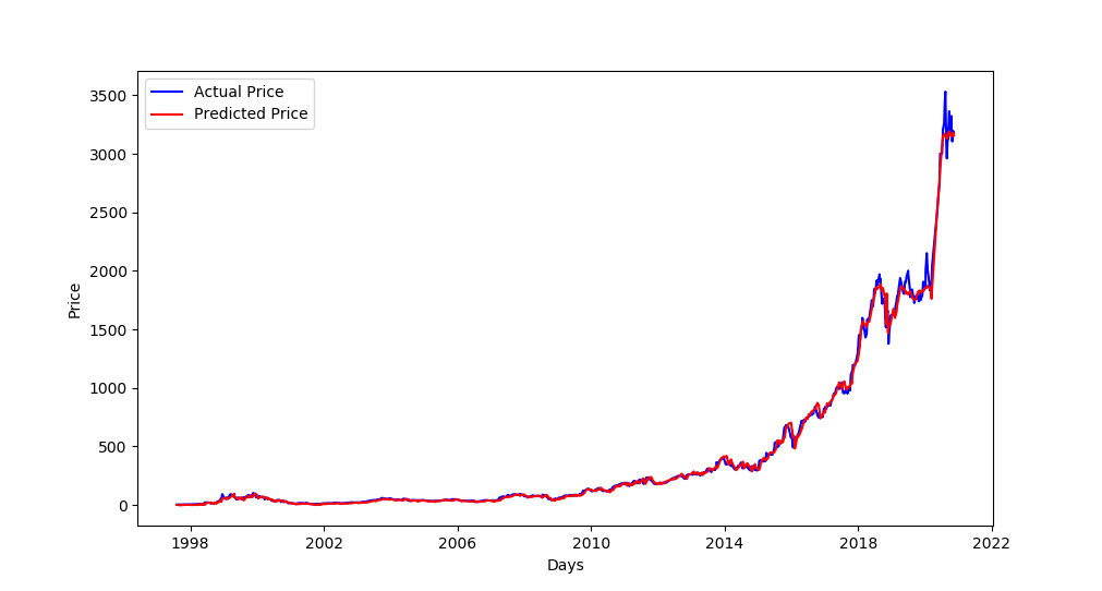
由于我们设置SPLIT_BY_DATE为False,该图显示了我们整个数据集上的测试集价差以及相应的预测价格(这解释了测试集在 1998 年之前开始)。
如果我们设置SPLIT_BY_DATE为True,则测试集将是TEST_SIZE总数据集的最后一个百分比(例如,如果我们有1997 年到2020 年的数据,并且TEST_SIZE为0.2,则测试样本的范围将在2016 年到2020 年左右)。
最后,让我们打印最终数据帧的最后10行,这样你就可以看到它的样子:
print(final_df.tail(10))
# save the final dataframe to csv-results folder
csv_results_folder = "csv-results"
if not os.path.isdir(csv_results_folder):
    os.mkdir(csv_results_folder)
csv_filename = os.path.join(csv_results_folder, model_name + ".csv")
final_df.to_csv(csv_filename)我们还将数据帧保存在csv-results文件夹中,有输出:
            open        high        low         close       adjclose    volume  ticker  adjclose_15 true_adjclose_15  buy_profit    sell_profit
2021-03-10	3098.449951	3116.459961	3030.050049	3057.639893	3057.639893	3012500	AMZN	3239.598633	3094.080078       36.440186     0.000000
2021-03-11	3104.010010	3131.780029	3082.929932	3113.590088	3113.590088	2776400	AMZN	3238.842773	3161.000000       47.409912     0.000000
2021-03-12	3075.000000	3098.979980	3045.500000	3089.489990	3089.489990	2421900	AMZN	3238.662598	3226.729980       137.239990    0.000000
2021-03-15	3074.570068	3082.239990	3032.090088	3081.679932	3081.679932	2913600	AMZN	3238.824219	3223.820068       142.140137    0.000000
2021-03-17	3073.219971	3173.050049	3070.219971	3135.729980	3135.729980	3118600	AMZN	3238.115234	3299.300049       163.570068    0.000000
2021-03-18	3101.000000	3116.629883	3025.000000	3027.989990	3027.989990	3649600	AMZN	3238.491943	3372.199951       344.209961    0.000000
2021-03-25	3072.989990	3109.780029	3037.139893	3046.260010	3046.260010	3563500	AMZN	3238.083740	3399.439941       353.179932    0.000000
2021-04-15	3371.000000	3397.000000	3352.000000	3379.090088	3379.090088	3233600	AMZN	3223.817627	3306.370117       0.000000      72.719971
2021-04-23	3319.100098	3375.000000	3308.500000	3340.879883	3340.879883	3192800	AMZN	3226.480957	3222.899902       0.000000      117.979980
2021-05-03	3484.729980	3486.649902	3372.699951	3386.489990	3386.489990	5875500	AMZN	3217.589844	3244.989990       0.000000      141.500000
数据框具有以下列:
- 我们的测试集及其功能(open、high、low、close、adjclose和volume列)。
adjclose_15: 是adjclose15 天后的预测价格(因为LOOKUP_STEP设置为15),使用我们的训练模型。true_adjclose_15: 是adjclose15 天后的真实价格,我们通过移动测试数据集得到。buy_profit:这是我们在当天买入股票时获得的利润,负利润意味着我们亏损(应该是卖出交易,我们买入)。sell_profit:这是我们在该日期出售股票时获得的利润。
Python TensorFlow 2和Keras预测股票价格总结
好的,这就是本教程的内容,你可以调整参数并查看如何提高模型性能,尝试在更多epochs上进行训练,比如700甚至更多,增加或减少BATCH_SIZE并查看是否会变得更好,或者使用N_STEPS和LOOKUP_STEPS看看哪种组合效果最好。
Python如何预测股票价格?你还可以更改模型参数,例如增加层数或LSTM单元的数量,甚至尝试使用GRU单元代替LSTM。
注意还有其他特征和指标可以使用,为了提高预测效果,通常会使用一些其他信息作为特征,例如技术指标、公司产品创新、利率、汇率、公共政策、网络、财经新闻甚至员工人数!
我鼓励你更改模型架构,尝试使用CNN或Seq2Seq模型,甚至在现有模型中添加双向 LSTM(设置BIDIRECTIONAL为True),看看你是否可以改进它!
此外,使用不同的股票市场,查看雅虎财经页面,看看你真正想要的是哪一个!
要使用完整Python预测股票价格示例代码,我鼓励你使用完整的 notebook或拆分为不同 Python 文件的完整代码。