Python TensorFlow实现皮肤癌检测 - 了解如何使用迁移学习构建一个模型,该模型能够使用 TensorFlow 2 在 Python 中对良性和恶性(黑色素瘤)皮肤病进行分类。
皮肤癌是皮肤细胞的异常生长,它是最常见的癌症之一,不幸的是,它可能会致命。好消息是,如果及早发现,你的皮肤科医生可以治疗它并完全消除它。
Python如何检测皮肤癌?使用深度学习和神经网络,我们将能够对良性和恶性皮肤病进行分类,这可能有助于医生在早期诊断癌症。在本教程中,我们将制作一个皮肤病分类器,尝试使用Python 中的TensorFlow框架仅从照片图像中区分良性(痣和脂溢性角化病)和恶性(黑色素瘤)皮肤病。
首先,让我们安装所需的库:
pip3 install tensorflow tensorflow_hub matplotlib seaborn numpy pandas sklearn imblearn
打开一个新笔记本(或Google Colab)并导入必要的模块:
import tensorflow as tf
import tensorflow_hub as hub
import matplotlib.pyplot as plt
import numpy as np
import pandas as pd
import seaborn as sns
from tensorflow.keras.utils import get_file
from sklearn.metrics import roc_curve, auc, confusion_matrix
from imblearn.metrics import sensitivity_score, specificity_score

import os
import glob
import zipfile
import random

# to get consistent results after multiple runs
tf.random.set_seed(7)
np.random.seed(7)
random.seed(7)

# 0 for benign, 1 for malignant
class_names = ["benign", "malignant"]
准备数据集
Python如何检测皮肤癌?对于本教程,我们将仅使用ISIC 档案数据集的一小部分,以下函数下载数据集并将其解压缩到一个新data文件夹中:
def download_and_extract_dataset():
  # dataset from https://github.com/udacity/dermatologist-ai
  # 5.3GB
  train_url = "https://s3-us-west-1.amazonaws.com/udacity-dlnfd/datasets/skin-cancer/train.zip"
  # 824.5MB
  valid_url = "https://s3-us-west-1.amazonaws.com/udacity-dlnfd/datasets/skin-cancer/valid.zip"
  # 5.1GB
  test_url  = "https://s3-us-west-1.amazonaws.com/udacity-dlnfd/datasets/skin-cancer/test.zip"
  for i, download_link in enumerate([valid_url, train_url, test_url]):
    temp_file = f"temp{i}.zip"
    data_dir = get_file(origin=download_link, fname=os.path.join(os.getcwd(), temp_file))
    print("Extracting", download_link)
    with zipfile.ZipFile(data_dir, "r") as z:
      z.extractall("data")
    # remove the temp file
    os.remove(temp_file)

# comment the below line if you already downloaded the dataset
download_and_extract_dataset()
Python TensorFlow检测皮肤癌示例:这将需要几分钟时间,具体取决于你的连接,之后data将出现包含训练、验证和测试集的文件夹。每组是一个文件夹,其中包含三类皮肤病图像(痣、脂溢性角化病和黑色素瘤)。
注意:当你的 Internet 连接速度较慢时,你可能难以使用上述 Python 函数下载数据集,在这种情况下,你应该下载并手动将其解压缩data到当前目录的文件夹中。
现在我们的机器中有数据集,让我们找到一种方法来标记这些图像,记住我们将只对良性和恶性皮肤病进行分类,因此我们需要将痣和脂溢性角化病标记为值 0,黑色素瘤标记为 1。
下面的单元格为每个集合生成一个元数据 CSV 文件,CSV 文件中的每一行都对应于图像的路径及其标签(0 或 1):
# preparing data
# generate CSV metadata file to read img paths and labels from it
def generate_csv(folder, label2int):
    folder_name = os.path.basename(folder)
    labels = list(label2int)
    # generate CSV file
    df = pd.DataFrame(columns=["filepath", "label"])
    i = 0
    for label in labels:
        print("Reading", os.path.join(folder, label, "*"))
        for filepath in glob.glob(os.path.join(folder, label, "*")):
            df.loc[i] = [filepath, label2int[label]]
            i += 1
    output_file = f"{folder_name}.csv"
    print("Saving", output_file)
    df.to_csv(output_file)

# generate CSV files for all data portions, labeling nevus and seborrheic keratosis
# as 0 (benign), and melanoma as 1 (malignant)
# you should replace "data" path to your extracted dataset path
# don't replace if you used download_and_extract_dataset() function
generate_csv("data/train", {"nevus": 0, "seborrheic_keratosis": 0, "melanoma": 1})
generate_csv("data/valid", {"nevus": 0, "seborrheic_keratosis": 0, "melanoma": 1})
generate_csv("data/test", {"nevus": 0, "seborrheic_keratosis": 0, "melanoma": 1})该generate_csv()函数接受2个参数,第一个是集合的路径,例如,如果你已经下载并提取了数据集"E:\datasets\skin-cancer",那么训练集应该是这样的"E:\datasets\skin-cancer\train".
第二个参数是一个字典,它将每个皮肤疾病类别映射到其对应的标签值(同样,0 代表良性,1 代表恶性)。
我做这样一个功能的原因是能够将它用于其他皮肤病分类(例如黑素细胞分类),因此你可以添加更多皮肤病并将其用于其他问题。
运行单元后,你会注意到 3 个 CSV 文件将出现在你的当前目录中。现在让我们使用tf.data API 中的from_tensor_slices()方法来加载这些元数据文件:
# loading data
train_metadata_filename = "train.csv"
valid_metadata_filename = "valid.csv"
# load CSV files as DataFrames
df_train = pd.read_csv(train_metadata_filename)
df_valid = pd.read_csv(valid_metadata_filename)
n_training_samples = len(df_train)
n_validation_samples = len(df_valid)
print("Number of training samples:", n_training_samples)
print("Number of validation samples:", n_validation_samples)
train_ds = tf.data.Dataset.from_tensor_slices((df_train["filepath"], df_train["label"]))
valid_ds = tf.data.Dataset.from_tensor_slices((df_valid["filepath"], df_valid["label"]))现在我们已经加载了数据集(train_ds和valid_ds),每个样本都是filepath(图像文件的路径)和label(0代表良性,1代表恶性)的元组,这里是输出:
Number of training samples: 2000
Number of validation samples: 150
复制让我们加载图像:
# preprocess data
def decode_img(img):
  # convert the compressed string to a 3D uint8 tensor
  img = tf.image.decode_jpeg(img, channels=3)
  # Use `convert_image_dtype` to convert to floats in the [0,1] range.
  img = tf.image.convert_image_dtype(img, tf.float32)
  # resize the image to the desired size.
  return tf.image.resize(img, [299, 299])


def process_path(filepath, label):
  # load the raw data from the file as a string
  img = tf.io.read_file(filepath)
  img = decode_img(img)
  return img, label


valid_ds = valid_ds.map(process_path)
train_ds = train_ds.map(process_path)
# test_ds = test_ds
for image, label in train_ds.take(1):
    print("Image shape:", image.shape)
    print("Label:", label.numpy())
Python TensorFlow实现皮肤癌检测:上面的代码使用map()方法process_path()在两组上的每个样本上执行函数,它基本上会加载图像,解码图像格式,将图像像素转换为范围内[0, 1]并将其调整为(299, 299, 3),然后我们拍摄一张图像并打印其形状:
Image shape: (299, 299, 3)
Label: 0
一切都如预期,现在让我们准备这个数据集进行训练:
# training parameters
batch_size = 64
optimizer = "rmsprop"

def prepare_for_training(ds, cache=True, batch_size=64, shuffle_buffer_size=1000):
  if cache:
    if isinstance(cache, str):
      ds = ds.cache(cache)
    else:
      ds = ds.cache()
  # shuffle the dataset
  ds = ds.shuffle(buffer_size=shuffle_buffer_size)
  # Repeat forever
  ds = ds.repeat()
  # split to batches
  ds = ds.batch(batch_size)
  # `prefetch` lets the dataset fetch batches in the background while the model
  # is training.
  ds = ds.prefetch(buffer_size=tf.data.experimental.AUTOTUNE)
  return ds

valid_ds = prepare_for_training(valid_ds, batch_size=batch_size, cache="valid-cached-data")
train_ds = prepare_for_training(train_ds, batch_size=batch_size, cache="train-cached-data")
这是我们所做的:
cache():由于我们对每个集合进行了太多计算,因此我们使用cache()方法将我们预处理的数据集保存到本地缓存文件中,这只会在第一次(在训练期间的第一个 epoch 中)对其进行预处理。shuffle():基本上是对数据集进行打乱,因此样本按随机顺序排列。repeat():每次我们迭代数据集时,它都会不断地为我们生成样本,这将在训练过程中帮助我们。batch():我们将每个训练步骤的数据集分成64或32 个样本。prefetch():这将使我们能够在模型训练时在后台获取批次。
Python TensorFlow检测皮肤癌示例:下面的单元格获取第一个验证批次并绘制图像及其相应的标签:
batch = next(iter(valid_ds))

def show_batch(batch):
  plt.figure(figsize=(12,12))
  for n in range(25):
      ax = plt.subplot(5,5,n+1)
      plt.imshow(batch[0][n])
      plt.title(class_names[batch[1][n].numpy()].title())
      plt.axis('off')

show_batch(batch)
输出:
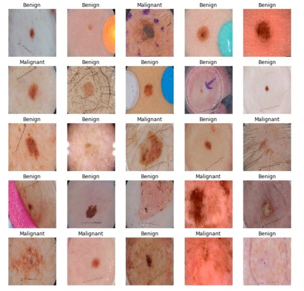
如你所见,区分恶性疾病和良性疾病极其困难,让我们看看我们的模型将如何处理它。
太好了,现在我们的数据集已经准备好了,让我们开始构建我们的模型。
构建模型
Python如何检测皮肤癌?前通知,我们调整所有图像(299, 299, 3),这是因为什么呢InceptionV3架构预计作为输入,因此我们将使用迁移学习与TensorFlow中心库下载并与其一起加载InceptionV3架构ImageNet预训练的权重:
# building the model
# InceptionV3 model & pre-trained weights
module_url = "https://tfhub.dev/google/tf2-preview/inception_v3/feature_vector/4"
m = tf.keras.Sequential([
    hub.KerasLayer(module_url, output_shape=[2048], trainable=False),
    tf.keras.layers.Dense(1, activation="sigmoid")
])

m.build([None, 299, 299, 3])
m.compile(loss="binary_crossentropy", optimizer=optimizer, metrics=["accuracy"])
m.summary()我们设置trainable为False因此我们将无法在训练期间调整预训练的权重,我们还添加了一个具有1 个单元的最终输出层,预计输出0到1之间的值(接近0表示良性,并且1为恶性)。
之后,由于这是一个二元分类,我们使用二元交叉熵损失构建我们的模型,并使用准确性作为我们的度量(不是那个可靠的度量,我们很快就会看到为什么),这是我们模型摘要的输出:
Model: "sequential"
_________________________________________________________________
Layer (type)                 Output Shape              Param #
=================================================================
keras_layer (KerasLayer)     multiple                  21802784
_________________________________________________________________
dense (Dense)                multiple                  2049
=================================================================
Total params: 21,804,833
Trainable params: 2,049
Non-trainable params: 21,802,784
_________________________________________________________________
训练模型
我们现在有了我们的数据集和模型,让我们把它们放在一起:
model_name = f"benign-vs-malignant_{batch_size}_{optimizer}"
tensorboard = tf.keras.callbacks.TensorBoard(log_dir=os.path.join("logs", model_name))
# saves model checkpoint whenever we reach better weights
modelcheckpoint = tf.keras.callbacks.ModelCheckpoint(model_name + "_{val_loss:.3f}.h5", save_best_only=True, verbose=1)

history = m.fit(train_ds, validation_data=valid_ds,
                steps_per_epoch=n_training_samples // batch_size,
                validation_steps=n_validation_samples // batch_size, verbose=1, epochs=100,
                callbacks=[tensorboard, modelcheckpoint])
复制我们使用ModelCheckpoint回调来保存迄今为止每个 epoch 的最佳权重,这就是我将epochs设置为100的原因,这是因为它可以随时收敛到更好的权重,以节省你的时间,随意将其减少到30或所以。
我还添加了tensorboard作为回调,以防你想尝试不同的超参数值。
由于fit()方法不知道数据集中的样本数量,我们需要分别指定训练集和验证集的迭代次数(样本数除以批量大小)steps_per_epoch和validation_steps参数。
这是训练期间输出的一部分:
Train for 31 steps, validate for 2 steps
Epoch 1/100
30/31 [============================>.] - ETA: 9s - loss: 0.4609 - accuracy: 0.7760
Epoch 00001: val_loss improved from inf to 0.49703, saving model to benign-vs-malignant_64_rmsprop_0.497.h5
31/31 [==============================] - 282s 9s/step - loss: 0.4646 - accuracy: 0.7722 - val_loss: 0.4970 - val_accuracy: 0.8125
<..SNIPED..>
Epoch 27/100
30/31 [============================>.] - ETA: 0s - loss: 0.2982 - accuracy: 0.8708
Epoch 00027: val_loss improved from 0.40253 to 0.38991, saving model to benign-vs-malignant_64_rmsprop_0.390.h5
31/31 [==============================] - 21s 691ms/step - loss: 0.3025 - accuracy: 0.8684 - val_loss: 0.3899 - val_accuracy: 0.8359
<..SNIPED..>
Epoch 41/100
30/31 [============================>.] - ETA: 0s - loss: 0.2800 - accuracy: 0.8802
Epoch 00041: val_loss did not improve from 0.38991
31/31 [==============================] - 21s 690ms/step - loss: 0.2829 - accuracy: 0.8790 - val_loss: 0.3948 - val_accuracy: 0.8281
Epoch 42/100
30/31 [============================>.] - ETA: 0s - loss: 0.2680 - accuracy: 0.8859
Epoch 00042: val_loss did not improve from 0.38991
31/31 [==============================] - 21s 693ms/step - loss: 0.2722 - accuracy: 0.8831 - val_loss: 0.4572 - val_accuracy: 0.8047
Python如何检测皮肤癌?模型评估
Python TensorFlow检测皮肤癌示例:首先,让我们像之前一样加载我们的测试集:
# evaluation
# load testing set
test_metadata_filename = "test.csv"
df_test = pd.read_csv(test_metadata_filename)
n_testing_samples = len(df_test)
print("Number of testing samples:", n_testing_samples)
test_ds = tf.data.Dataset.from_tensor_slices((df_test["filepath"], df_test["label"]))

def prepare_for_testing(ds, cache=True, shuffle_buffer_size=1000):
  if cache:
    if isinstance(cache, str):
      ds = ds.cache(cache)
    else:
      ds = ds.cache()
  ds = ds.shuffle(buffer_size=shuffle_buffer_size)
  return ds

test_ds = test_ds.map(process_path)
test_ds = prepare_for_testing(test_ds, cache="test-cached-data")
上面的代码加载我们的测试数据并准备测试:
Number of testing samples: 600600形状的图像(299, 299, 3)可以适合我们的记忆,让我们将测试集从tf.data转换为 NumPy 数组:
# convert testing set to numpy array to fit in memory (don't do that when testing
# set is too large)
y_test = np.zeros((n_testing_samples,))
X_test = np.zeros((n_testing_samples, 299, 299, 3))
for i, (img, label) in enumerate(test_ds.take(n_testing_samples)):
  # print(img.shape, label.shape)
  X_test[i] = img
  y_test[i] = label.numpy()

print("y_test.shape:", y_test.shape)上面的单元格将构造我们的数组,第一次执行它需要一些时间,因为它正在执行process_path()和prepare_for_testing()函数中定义的所有预处理。
现在让我们加载ModelCheckpoint在训练期间保存的最佳权重:
# load the weights with the least loss
m.load_weights("benign-vs-malignant_64_rmsprop_0.390.h5")
你可能没有最佳权重的确切文件名,你需要在当前目录中搜索损失最小的保存权重,以下代码使用精度指标评估模型:
print("Evaluating the model...")
loss, accuracy = m.evaluate(X_test, y_test, verbose=0)
print("Loss:", loss, "  Accuracy:", accuracy)
输出:
Evaluating the model...
Loss: 0.4476394319534302   Accuracy: 0.8
Python TensorFlow实现皮肤癌检测:我们已经达到84%了验证集和80%测试集的准确性,但这还不是全部。由于我们的数据集在很大程度上是不平衡的,因此准确性并不能说明一切。事实上,将每张图像预测为良性的模型的准确度为80%,因为恶性样本约占总验证集的 20%。
因此,我们需要一种更好的方法来评估我们的模型,在即将到来的单元格中,我们将使用seaborn和matplotlib库来绘制混淆矩阵,它告诉我们更多关于我们的模型表现如何。但在我们这样做之前,我只想说清楚:我们都知道将恶性疾病预测为良性是一个可怕的错误,这样做可以杀死人!所以我们需要一种方法来预测更多的恶性病例,即使与良性相比,我们的恶性样本很少。一个好的方法是引入一个阈值。
请记住,神经网络的输出是一个介于0和1之间的值。在正常情况下,当神经网络产生0到0.5之间的值时,我们会自动将其指定为良性,将0.5到1.0 指定为恶性。因为我们想知道我们可以将恶性疾病预测为良性这一事实(这只是众多原因之一),我们可以说,例如,从0到0.3是良性的,从0.3到1.0是恶性的,这意味着我们使用的阈值为 0.3,这将改善我们的预测。
下面的函数可以做到这一点:
def get_predictions(threshold=None):
  """
  Returns predictions for binary classification given `threshold`
  For instance, if threshold is 0.3, then it'll output 1 (malignant) for that sample if
  the probability of 1 is 30% or more (instead of 50%)
  """
  y_pred = m.predict(X_test)
  if not threshold:
    threshold = 0.5
  result = np.zeros((n_testing_samples,))
  for i in range(n_testing_samples):
    # test melanoma probability
    if y_pred[i][0] >= threshold:
      result[i] = 1
    # else, it's 0 (benign)
  return result

threshold = 0.23
# get predictions with 23% threshold
# which means if the model is 23% sure or more that is malignant,
# it's assigned as malignant, otherwise it's benign
y_pred = get_predictions(threshold)
现在让我们绘制混淆矩阵并解释它:
def plot_confusion_matrix(y_test, y_pred):
  cmn = confusion_matrix(y_test, y_pred)
  # Normalise
  cmn = cmn.astype('float') / cmn.sum(axis=1)[:, np.newaxis]
  # print it
  print(cmn)
  fig, ax = plt.subplots(figsize=(10,10))
  sns.heatmap(cmn, annot=True, fmt='.2f',
              xticklabels=[f"pred_{c}" for c in class_names],
              yticklabels=[f"true_{c}" for c in class_names],
              cmap="Blues"
              )
  plt.ylabel('Actual')
  plt.xlabel('Predicted')
  # plot the resulting confusion matrix
  plt.show()

plot_confusion_matrix(y_test, y_pred)
输出:
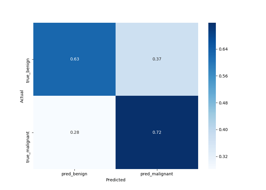
灵敏度
因此0.72,鉴于患者患有疾病(混淆矩阵的右下角),我们的模型获得了阳性测试的概率,这通常称为敏感性。
灵敏度是一种广泛用于医学的统计量度,由以下公式给出(来自维基百科):

72%他们是恶性的,还不错,但需要改进。
特异性
另一个指标是特异性,你可以在混淆矩阵的左上角阅读它,我们得到了63%. 考虑到患者身体状况良好,基本上是阴性测试的概率:

63%他们是良性的。
由于具有高特异性,该测试很少在健康患者中给出阳性结果,而高灵敏度意味着该模型在其结果为阴性时是可靠的,我邀请你在这篇维基百科文章中阅读更多相关信息。
或者,你可以使用imblearn模块来获得这些分数:
sensitivity = sensitivity_score(y_test, y_pred)
specificity = specificity_score(y_test, y_pred)

print("Melanoma Sensitivity:", sensitivity)
print("Melanoma Specificity:", specificity)
输出:
Melanoma Sensitivity: 0.717948717948718
Melanoma Specificity: 0.6252587991718427
接收器工作特性
Python TensorFlow检测皮肤癌示例:另一个很好的度量是ROC,这基本上是一个曲线图昭示着我们我们的二元分类的诊断能力,它的功能在A真阳性率Y轴和对假阳性率X轴。我们想要达到的完美点位于图的左上角,这是使用matplotlib绘制 ROC 曲线的代码:
def plot_roc_auc(y_true, y_pred):
    """
    This function plots the ROC curves and provides the scores.
    """
    # prepare for figure
    plt.figure()
    fpr, tpr, _ = roc_curve(y_true, y_pred)
    # obtain ROC AUC
    roc_auc = auc(fpr, tpr)
    # print score
    print(f"ROC AUC: {roc_auc:.3f}")
    # plot ROC curve
    plt.plot(fpr, tpr, color="blue", lw=2,
                label='ROC curve (area = {f:.2f})'.format(d=1, f=roc_auc))
    plt.xlim([0.0, 1.0])
    plt.ylim([0.0, 1.05])
    plt.xlabel('False Positive Rate')
    plt.ylabel('True Positive Rate')
    plt.title('ROC curves')
    plt.legend(loc="lower right")
    plt.show()

plot_roc_auc(y_test, y_pred)
输出:
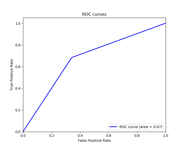
ROC AUC: 0.671太棒了,因为我们想最大化真阳性率,最小化假阳性率,计算 ROC 曲线下面积证明是有用的,我们得到 0.671 作为曲线下面积 ROC (ROC AUC),面积为 1 意味着该模型适用于所有情况。
Python TensorFlow实现皮肤癌检测总结
Python如何检测皮肤癌?我们完成了!有了它,看看你如何改进模型,我们只使用了2000训练样本,去ISIC 存档并下载更多并将它们添加到data文件夹中,分数将根据你添加的样本数量显着提高。你可以使用ISIC 档案下载器,它可以帮助你以你想要的方式下载数据集。
我还鼓励你调整超参数,例如我们之前设置的阈值,看看你是否可以获得更好的灵敏度和特异性分数。
我使用了InceptionV3模型架构,你可以随意使用任何你想要的 CNN 架构,我邀请你浏览TensorFlow hub并选择最新的模型。