python如何识别猫狗？对狗和猫的照片进行分类（准确率为 97%）

逐步开发深度卷积神经网络以对狗和猫的照片进行分类

Dogs vs. Cats 数据集是一个标准的计算机视觉数据集，涉及将照片分类为包含狗或猫。

python如何识别猫狗？尽管这个问题听起来很简单，但直到最近几年才使用深度学习卷积神经网络有效地解决了这个问题。在有效解决数据集的同时，它可以作为学习和实践如何从头开始开发、评估和使用卷积深度学习神经网络进行图像分类的基础。

这包括如何开发一个强大的测试工具来估计模型的性能，如何探索模型的改进，以及如何保存模型并稍后加载它以对新数据进行预测。

在本教程中，你将了解如何开发卷积神经网络来对狗和猫的照片进行分类。

完成本教程后，你将了解：

• 如何加载和准备用于建模的狗和猫的照片。
• 如何从头开发用于照片分类的卷积神经网络并提高模型性能。
• 如何使用迁移学习开发照片分类模型。

使用我的新书Deep Learning for Computer Vision启动你的项目，包括分步教程和所有示例的Python 源代码文件。

让我们开始吧。

• 2019 年 10 月更新：针对 Keras 2.3 和 TensorFlow 2.0 更新。

如何开发卷积神经网络对狗和猫的
照片进行分类Cohen Van der Velde照片，保留部分权利。

教程概述

本教程分为六个部分；他们是：

1. 狗与猫的预测问题
2. 狗 vs. 猫数据集准备
3. 开发基线 CNN 模型
4. 开发模型改进
5. 探索迁移学习
6. 如何完成模型并进行预测

狗与猫的预测问题

狗 vs 猫数据集是指用于 2013 年举行的 Kaggle 机器学习竞赛的数据集。

该数据集由狗和猫的照片组成，作为来自 300 万张手动注释照片的更大数据集的照片子集提供。该数据集是作为 Petfinder.com 和 Microsoft 之间的合作伙伴关系开发的。

该数据集最初用作 CAPTCHA（或完全自动化的公共图灵测试，以区分计算机和人类），即认为人类认为微不足道但机器无法解决的任务，用于网站上区分在人类用户和机器人之间。具体来说，该任务被称为“ Asirra ”或用于限制访问的动物物种图像识别，一种 CAPTCHA。该任务在 2007 年题为“ Asirra: A CAPTCHA that Exploits Interest-Aligned Manual Image Categorization ”中有所描述。

我们展示了 Asirra，这是一个 CAPTCHA，它要求用户从一组 12 张猫和狗的照片中识别出猫。Asirra 对用户来说很容易；用户研究表明，人类可以在 30 秒内解决 99.6% 的问题。除非机器视觉取得重大进展，否则我们预计计算机解决它的机会不会超过 1/54,000。

— Asirra：利用兴趣对齐的手动图像分类的验证码，2007 年。

在比赛发布时，使用 SVM 实现了最先进的结果，并在 2007 年一篇题为“机器学习攻击 Asirra CAPTCHA ”（PDF）的论文中进行了描述，该结果实现了 80% 的分类准确率. 正是这篇论文证明了该任务在提出该任务后不久就不再适合 CAPTCHA 任务。

……我们描述了一个分类器，它在区分 Asirra 中使用的猫和狗的图像时准确率为 82.7%。该分类器是对从图像中提取的颜色和纹理特征进行训练的支持向量机分类器的组合。[...] 我们的结果表明，不要在没有保护措施的情况下部署 Asirra。

—机器学习攻击 Asirra CAPTCHA，2007 年。

python识别猫狗的方法 - Kaggle 比赛提供了 25,000 张标记照片：12,500 只狗和相同数量的猫。然后需要对包含 12,500 张未标记照片的测试数据集进行预测。Pierre Sermanet（目前是 Google Brain 的研究科学家）赢得了比赛，他在测试数据集的 70% 子样本上实现了约 98.914% 的分类准确率。他的方法后来被描述为 2013 年题为“ OverFeat：使用卷积网络的集成识别、定位和检测”的论文的一部分。

该数据集易于理解且小到足以放入内存。因此，它已成为初学者开始使用卷积神经网络时的一个很好的“ hello world ”或“入门”计算机视觉数据集。

因此，使用手动设计的卷积神经网络实现大约 80% 的准确度和使用迁移学习在此任务上实现90% 以上的准确度是常规的。

狗 vs. 猫数据集准备

对狗和猫的照片进行分类：该数据集可以从 Kaggle 网站免费下载，但我相信你必须拥有一个 Kaggle 帐户。

如果你没有 Kaggle 帐户，请先注册。

通过访问 Dogs vs. Cats Data 页面下载数据集，然后单击“全部下载”按钮。

这会将 850 兆字节的文件“ dogs-vs-cats.zip ”下载到你的工作站。

解压缩文件，你将看到train.zip、train1.zip和一个.csv文件。解压缩train.zip文件，因为我们将只关注这个数据集。

你现在将拥有一个名为“ train/ ”的文件夹，其中包含 25,000 个狗和猫的 .jpg 文件。照片按文件名标记，带有“狗”或“猫”字样。文件命名约定如下：

cat.0.jpg
...
cat.124999.jpg
dog.0.jpg
dog.124999.jpg

绘制狗和猫的照片

随意查看目录中的几张照片，可以看到照片都是彩色的，而且形状和大小各不相同。

例如，让我们在一个图中加载和绘制狗的前九张照片。

下面列出了完整的示例。

# plot dog photos from the dogs vs cats dataset
from matplotlib import pyplot
from matplotlib.image import imread
# define location of dataset
folder = 'train/'
# plot first few images
for i in range(9):
	# define subplot
	pyplot.subplot(330 + 1 + i)
	# define filename
	filename = folder + 'dog.' + str(i) + '.jpg'
	# load image pixels
	image = imread(filename)
	# plot raw pixel data
	pyplot.imshow(image)
# show the figure
pyplot.show()

运行该示例创建一个图形，显示数据集中狗的前九张照片。

我们可以看到，有些照片是横向格式，有些是纵向格式，还有一些是正方形。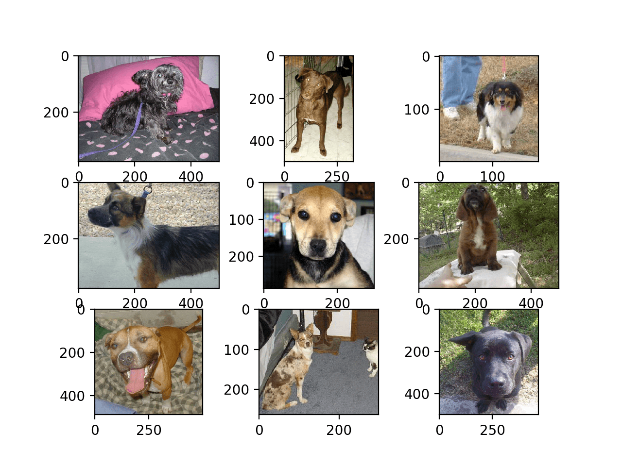

Dogs vs Cats 数据集中狗的前九张照片的图

python识别猫狗示例 - 我们可以更新示例并将其更改为绘制猫照片；下面列出了完整的示例。

# plot cat photos from the dogs vs cats dataset
from matplotlib import pyplot
from matplotlib.image import imread
# define location of dataset
folder = 'train/'
# plot first few images
for i in range(9):
	# define subplot
	pyplot.subplot(330 + 1 + i)
	# define filename
	filename = folder + 'cat.' + str(i) + '.jpg'
	# load image pixels
	image = imread(filename)
	# plot raw pixel data
	pyplot.imshow(image)
# show the figure
pyplot.show()

同样，我们可以看到照片都是不同的尺寸。

我们还可以看到一张照片，其中猫几乎看不见（左下角），另一张有两只猫（右下角）。这表明任何适合这个问题的分类器都必须是稳健的。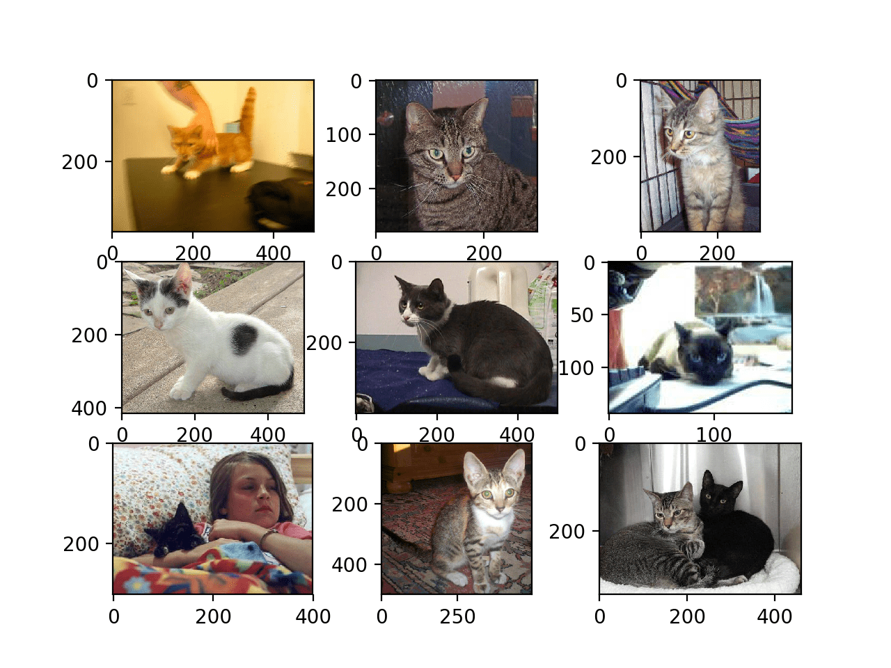

Dogs vs Cats 数据集中前九张猫照片的图

选择标准照片尺寸

在建模之前必须对照片进行重新整形，以便所有图像都具有相同的形状。这通常是一个小的方形图像。

有很多方法可以实现这一点，尽管最常见的是简单的调整大小操作，它会拉伸和变形每个图像的纵横比并强制其变成新的形状。

我们可以加载所有照片并查看照片宽度和高度的分布，然后设计一个最能反映我们在实践中最有可能看到的新照片尺寸。

较小的输入意味着模型可以更快地训练，并且通常这种关注支配着图像大小的选择。在这种情况下，我们将遵循这种方法并选择 200×200 像素的固定大小。

预处理照片尺寸（可选）

如果我们想将所有图像加载到内存中，我们可以估计它需要大约 12 GB 的 RAM。

即 25,000 张图像，每个图像具有 200x200x3 像素，或 3,000,000,000 个 32 位像素值。

我们可以加载所有图像，重塑它们，并将它们存储为单个 NumPy 数组。这可以适合许多现代机器上的 RAM，但不是全部，特别是如果你只有 8 GB 可以使用。

我们可以编写自定义代码将图像加载到内存中，并在加载过程中调整它们的大小，然后保存它们以备建模。

下面的示例使用 Keras 图像处理 API 加载训练数据集中的所有 25,000 张照片并将它们重塑为 200×200 方形照片。标签也是根据文件名为每张照片确定的。然后保存一组照片和标签。

# load dogs vs cats dataset, reshape and save to a new file
from os import listdir
from numpy import asarray
from numpy import save
from keras.preprocessing.image import load_img
from keras.preprocessing.image import img_to_array
# define location of dataset
folder = 'train/'
photos, labels = list(), list()
# enumerate files in the directory
for file in listdir(folder):
	# determine class
	output = 0.0
	if file.startswith('cat'):
		output = 1.0
	# load image
	photo = load_img(folder + file, target_size=(200, 200))
	# convert to numpy array
	photo = img_to_array(photo)
	# store
	photos.append(photo)
	labels.append(output)
# convert to a numpy arrays
photos = asarray(photos)
labels = asarray(labels)
print(photos.shape, labels.shape)
# save the reshaped photos
save('dogs_vs_cats_photos.npy', photos)
save('dogs_vs_cats_labels.npy', labels)

运行该示例可能需要大约一分钟的时间将所有图像加载到内存中并打印加载数据的形状以确认它已正确加载。

注意：运行此示例假定你有超过 12 GB 的 RAM。如果你没有足够的内存，你可以跳过这个例子；它仅作为演示提供。

(25000, 200, 200, 3) (25000,)

在运行结束时，会创建两个名为“ dogs_vs_cats_photos.npy ”和“ dogs_vs_cats_labels.npy ”的文件，其中包含所有调整大小的图像及其关联的类标签。这些文件加在一起只有大约 12 GB 的大小，并且加载速度明显快于单个图像。

准备好的数据可以直接加载；例如：

# load and confirm the shape
from numpy import load
photos = load('dogs_vs_cats_photos.npy')
labels = load('dogs_vs_cats_labels.npy')
print(photos.shape, labels.shape)

将照片预处理为标准目录

或者，我们可以使用Keras ImageDataGenerator 类和flow_from_directory() API逐步加载图像。这执行起来会更慢，但会在更多机器上运行。

这个API更喜欢将数据分成单独的train/和test/目录，每个目录下每个类都有一个子目录，例如一个train/dog/和一个train/cat/子目录，test也一样。然后在子目录下组织图像。

我们可以编写一个脚本来创建具有这种首选结构的数据集的副本。我们将随机选择 25% 的图像（或 6,250 个）用于测试数据集。

首先，我们需要创建如下目录结构：

dataset_dogs_vs_cats
├── test
│   ├── cats
│   └── dogs
└── train
    ├── cats
    └── dogs

我们可以使用makedirs()函数在 Python 中创建目录，并使用循环为train/和test/目录创建dog/和cat/子目录。

# create directories
dataset_home = 'dataset_dogs_vs_cats/'
subdirs = ['train/', 'test/']
for subdir in subdirs:
	# create label subdirectories
	labeldirs = ['dogs/', 'cats/']
	for labldir in labeldirs:
		newdir = dataset_home + subdir + labldir
		makedirs(newdir, exist_ok=True)

接下来，我们可以枚举数据集中的所有图像文件，并根据文件名将它们复制到dog/或cats/子目录中。

此外，我们可以随机决定将 25% 的图像保留到测试数据集中。这是通过固定伪随机数生成器的种子来一致地完成的，这样每次运行代码时我们都会得到相同的数据分割。

# seed random number generator
seed(1)
# define ratio of pictures to use for validation
val_ratio = 0.25
# copy training dataset images into subdirectories
src_directory = 'train/'
for file in listdir(src_directory):
	src = src_directory + '/' + file
	dst_dir = 'train/'
	if random() < val_ratio:
		dst_dir = 'test/'
	if file.startswith('cat'):
		dst = dataset_home + dst_dir + 'cats/'  + file
		copyfile(src, dst)
	elif file.startswith('dog'):
		dst = dataset_home + dst_dir + 'dogs/'  + file
		copyfile(src, dst)

下面列出了完整的代码示例，并假设你已将下载的train.zip 中的图像解压缩到当前工作目录中的train/ 中。

# organize dataset into a useful structure
from os import makedirs
from os import listdir
from shutil import copyfile
from random import seed
from random import random
# create directories
dataset_home = 'dataset_dogs_vs_cats/'
subdirs = ['train/', 'test/']
for subdir in subdirs:
	# create label subdirectories
	labeldirs = ['dogs/', 'cats/']
	for labldir in labeldirs:
		newdir = dataset_home + subdir + labldir
		makedirs(newdir, exist_ok=True)
# seed random number generator
seed(1)
# define ratio of pictures to use for validation
val_ratio = 0.25
# copy training dataset images into subdirectories
src_directory = 'train/'
for file in listdir(src_directory):
	src = src_directory + '/' + file
	dst_dir = 'train/'
	if random() < val_ratio:
		dst_dir = 'test/'
	if file.startswith('cat'):
		dst = dataset_home + dst_dir + 'cats/'  + file
		copyfile(src, dst)
	elif file.startswith('dog'):
		dst = dataset_home + dst_dir + 'dogs/'  + file
		copyfile(src, dst)

运行该示例后，你现在将拥有一个新的dataset_dogs_vs_cats/目录，其中包含一个train/和val/子文件夹以及更多dog/ can cats/子目录，与设计完全一样。

开发基线 CNN 模型

在本节中，我们可以为狗与猫数据集开发一个基线卷积神经网络模型。

基线模型将建立一个最低模型性能，我们所有其他模型都可以与之进行比较，以及一个模型架构，我们可以将其用作研究和改进的基础。

一个好的起点是 VGG 模型的一般架构原则。这是一个很好的起点，因为它们在 ILSVRC 2014 竞赛中取得了顶级性能，并且架构的模块化结构易于理解和实现。有关 VGG 模型的更多详细信息，请参阅 2015 年的论文“ Very Deep Convolutional Networks for Large-Scale Image Recognition”。

该架构涉及用小的 3×3 过滤器堆叠卷积层，然后是最大池化层。这些层一起形成一个块，这些块可以重复，其中每个块中的过滤器数量随着网络的深度而增加，例如模型的前四个块的 32、64、128、256。填充用于卷积层以确保输出特征图的高度和宽度形状与输入匹配。

python如何识别猫狗？我们可以在狗与猫的问题上探索这种架构，并将具有 1、2 和 3 个块的这种架构的模型进行比较。

每一层都会使用ReLU 激活函数和 He 权重初始化，这通常是最佳实践。例如，可以在 Keras 中定义一个 3 块 VGG 风格的架构，其中每个块都有一个卷积和池化层，如下所示：

# block 1
model.add(Conv2D(32, (3, 3), activation='relu', kernel_initializer='he_uniform', padding='same', input_shape=(200, 200, 3)))
model.add(MaxPooling2D((2, 2)))
# block 2
model.add(Conv2D(64, (3, 3), activation='relu', kernel_initializer='he_uniform', padding='same'))
model.add(MaxPooling2D((2, 2)))
# block 3
model.add(Conv2D(128, (3, 3), activation='relu', kernel_initializer='he_uniform', padding='same'))
model.add(MaxPooling2D((2, 2)))

我们可以创建一个名为define_model()的函数，该函数将定义一个模型并返回它准备好适合数据集。然后可以自定义此函数以定义不同的基线模型，例如具有 1、2 或 3 个 VGG 样式块的模型版本。

该模型将适合随机梯度下降，我们将从 0.001 的保守学习率和 0.9 的动量开始。

该问题是一项二元分类任务，需要预测 0 或 1 中的一个值。将使用具有 1 个节点和 sigmoid 激活的输出层，并将使用二元交叉熵损失函数优化模型。

下面是一个define_model()函数的示例，该函数使用一个 vgg 样式块为狗与猫问题定义卷积神经网络模型。

# define cnn model
def define_model():
	model = Sequential()
	model.add(Conv2D(32, (3, 3), activation='relu', kernel_initializer='he_uniform', padding='same', input_shape=(200, 200, 3)))
	model.add(MaxPooling2D((2, 2)))
	model.add(Flatten())
	model.add(Dense(128, activation='relu', kernel_initializer='he_uniform'))
	model.add(Dense(1, activation='sigmoid'))
	# compile model
	opt = SGD(lr=0.001, momentum=0.9)
	model.compile(optimizer=opt, loss='binary_crossentropy', metrics=['accuracy'])
	return model

可以根据需要调用它来准备模型，例如：

# define model
model = define_model()

接下来，我们需要准备数据。

这涉及首先定义一个ImageDataGenerator实例，它将像素值缩放到 0-1 的范围。

# create data generator
datagen = ImageDataGenerator(rescale=1.0/255.0)

接下来，需要为训练和测试数据集准备迭代器。

我们可以在数据生成器上使用flow_from_directory()函数，并为每个train/和test/目录创建一个迭代器。我们必须通过“ class_mode ”参数指定问题是二分类问题，并通过“ target_size ”参数加载大小为200×200像素的图像。我们将批量大小固定为 64。

# prepare iterators
train_it = datagen.flow_from_directory('dataset_dogs_vs_cats/train/',
	class_mode='binary', batch_size=64, target_size=(200, 200))
test_it = datagen.flow_from_directory('dataset_dogs_vs_cats/test/',
	class_mode='binary', batch_size=64, target_size=(200, 200))

然后，我们可以使用训练迭代器 ( train_it )拟合模型，并在训练期间使用测试迭代器 ( test_it ) 作为验证数据集。

必须指定训练和测试迭代器的步数。这是将构成一个时期的批次数。这可以通过每个迭代器的长度来指定，并且将是训练和测试目录中的图像总数除以批量大小 (64)。

该模型将适合 20 个 epoch，这是一个检查模型是否可以学习问题的少量数据。

# fit model
history = model.fit_generator(train_it, steps_per_epoch=len(train_it),
	validation_data=test_it, validation_steps=len(test_it), epochs=20, verbose=0)

拟合后，可以直接在测试数据集上评估最终模型并报告分类准确率。

# evaluate model
_, acc = model.evaluate_generator(test_it, steps=len(test_it), verbose=0)
print('> %.3f' % (acc * 100.0))

最后，我们可以创建存储在从调用fit_generator()返回的“ history ”目录中的训练期间收集的历史记录图。

History 包含每个 epoch 结束时测试和训练数据集上的模型准确性和损失。这些度量在训练时期的线图提供了学习曲线，我们可以使用它来了解模型是过度拟合、欠拟合还是拟合良好。

下面的summary_diagnostics()函数获取历史目录并创建一个带有损失线图和另一个用于准确性的线图的单一图形。然后将图形保存到文件中，文件名基于脚本名称。如果我们希望评估不同文件中模型的许多变体并为每个变体自动创建线图，这将很有帮助。

# plot diagnostic learning curves
def summarize_diagnostics(history):
	# plot loss
	pyplot.subplot(211)
	pyplot.title('Cross Entropy Loss')
	pyplot.plot(history.history['loss'], color='blue', label='train')
	pyplot.plot(history.history['val_loss'], color='orange', label='test')
	# plot accuracy
	pyplot.subplot(212)
	pyplot.title('Classification Accuracy')
	pyplot.plot(history.history['accuracy'], color='blue', label='train')
	pyplot.plot(history.history['val_accuracy'], color='orange', label='test')
	# save plot to file
	filename = sys.argv[0].split('/')[-1]
	pyplot.savefig(filename + '_plot.png')
	pyplot.close()

我们可以将所有这些结合到一个简单的测试工具中，用于测试模型配置。

下面列出了在狗和猫数据集上评估单块基线模型的完整python识别猫狗示例。

# baseline model for the dogs vs cats dataset
import sys
from matplotlib import pyplot
from keras.utils import to_categorical
from keras.models import Sequential
from keras.layers import Conv2D
from keras.layers import MaxPooling2D
from keras.layers import Dense
from keras.layers import Flatten
from keras.optimizers import SGD
from keras.preprocessing.image import ImageDataGenerator

# define cnn model
def define_model():
	model = Sequential()
	model.add(Conv2D(32, (3, 3), activation='relu', kernel_initializer='he_uniform', padding='same', input_shape=(200, 200, 3)))
	model.add(MaxPooling2D((2, 2)))
	model.add(Flatten())
	model.add(Dense(128, activation='relu', kernel_initializer='he_uniform'))
	model.add(Dense(1, activation='sigmoid'))
	# compile model
	opt = SGD(lr=0.001, momentum=0.9)
	model.compile(optimizer=opt, loss='binary_crossentropy', metrics=['accuracy'])
	return model

# plot diagnostic learning curves
def summarize_diagnostics(history):
	# plot loss
	pyplot.subplot(211)
	pyplot.title('Cross Entropy Loss')
	pyplot.plot(history.history['loss'], color='blue', label='train')
	pyplot.plot(history.history['val_loss'], color='orange', label='test')
	# plot accuracy
	pyplot.subplot(212)
	pyplot.title('Classification Accuracy')
	pyplot.plot(history.history['accuracy'], color='blue', label='train')
	pyplot.plot(history.history['val_accuracy'], color='orange', label='test')
	# save plot to file
	filename = sys.argv[0].split('/')[-1]
	pyplot.savefig(filename + '_plot.png')
	pyplot.close()

# run the test harness for evaluating a model
def run_test_harness():
	# define model
	model = define_model()
	# create data generator
	datagen = ImageDataGenerator(rescale=1.0/255.0)
	# prepare iterators
	train_it = datagen.flow_from_directory('dataset_dogs_vs_cats/train/',
		class_mode='binary', batch_size=64, target_size=(200, 200))
	test_it = datagen.flow_from_directory('dataset_dogs_vs_cats/test/',
		class_mode='binary', batch_size=64, target_size=(200, 200))
	# fit model
	history = model.fit_generator(train_it, steps_per_epoch=len(train_it),
		validation_data=test_it, validation_steps=len(test_it), epochs=20, verbose=0)
	# evaluate model
	_, acc = model.evaluate_generator(test_it, steps=len(test_it), verbose=0)
	print('> %.3f' % (acc * 100.0))
	# learning curves
	summarize_diagnostics(history)

# entry point, run the test harness
run_test_harness()

现在我们有了一个测试工具，让我们看一下对三个简单基线模型的评估。

单块 VGG 模型

单块 VGG 模型有一个带有 32 个过滤器的单个卷积层，后跟一个最大池化层。

该模型的define_model()函数在上一节中定义，但为了完整性在下面再次提供。

# define cnn model
def define_model():
	model = Sequential()
	model.add(Conv2D(32, (3, 3), activation='relu', kernel_initializer='he_uniform', padding='same', input_shape=(200, 200, 3)))
	model.add(MaxPooling2D((2, 2)))
	model.add(Flatten())
	model.add(Dense(128, activation='relu', kernel_initializer='he_uniform'))
	model.add(Dense(1, activation='sigmoid'))
	# compile model
	opt = SGD(lr=0.001, momentum=0.9)
	model.compile(optimizer=opt, loss='binary_crossentropy', metrics=['accuracy'])
	return model

运行此示例首先打印训练和测试数据集的大小，确认数据集已正确加载。

然后对模型进行拟合和评估，在现代 GPU 硬件上大约需要 20 分钟。

Found 18697 images belonging to 2 classes.
Found 6303 images belonging to 2 classes.
> 72.331

注意：你的结果可能会因算法或评估程序的随机性或数值精度的差异而有所不同。考虑多次运行该示例并比较平均结果。

在这种情况下，我们可以看到模型在测试数据集上达到了大约 72% 的准确率。

还创建了一个图，显示了损失的线图和模型在训练（蓝色）和测试（橙色）数据集上的准确性的线图。

查看此图，我们可以看到该模型在大约 12 个 epoch 时过度拟合了训练数据集。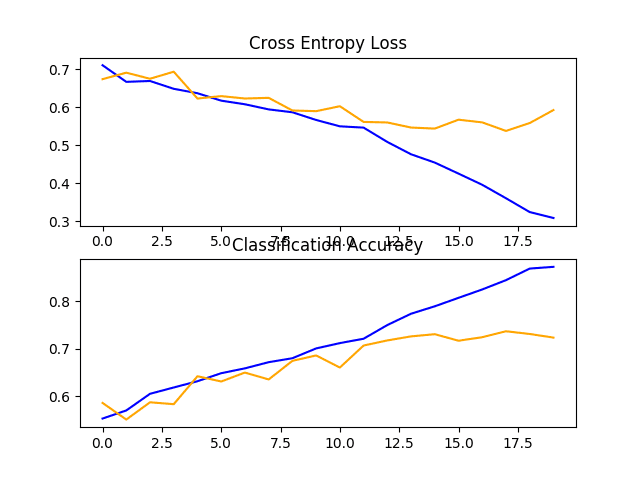

狗和猫数据集上带有一个 VGG 块的基线模型的损失和准确度学习曲线的线图

对狗和猫的照片进行分类：两块 VGG 模型

双块 VGG 模型扩展了单块模型并添加了具有 64 个过滤器的第二个块。

为了完整起见，下面提供了此模型的define_model()函数。

# define cnn model
def define_model():
	model = Sequential()
	model.add(Conv2D(32, (3, 3), activation='relu', kernel_initializer='he_uniform', padding='same', input_shape=(200, 200, 3)))
	model.add(MaxPooling2D((2, 2)))
	model.add(Conv2D(64, (3, 3), activation='relu', kernel_initializer='he_uniform', padding='same'))
	model.add(MaxPooling2D((2, 2)))
	model.add(Flatten())
	model.add(Dense(128, activation='relu', kernel_initializer='he_uniform'))
	model.add(Dense(1, activation='sigmoid'))
	# compile model
	opt = SGD(lr=0.001, momentum=0.9)
	model.compile(optimizer=opt, loss='binary_crossentropy', metrics=['accuracy'])
	return model

再次运行此示例将打印训练和测试数据集的大小，确认数据集已正确加载。

对模型进行拟合和评估，并报告在测试数据集上的性能。

Found 18697 images belonging to 2 classes.
Found 6303 images belonging to 2 classes.
> 76.646

注意：你的结果可能会因算法或评估程序的随机性或数值精度的差异而有所不同。考虑多次运行该示例并比较平均结果。

在这种情况下，我们可以看到模型实现了性能的小幅提升，从一个块的约 72% 到两个块的约 76% 的准确率

查看学习曲线图，我们可以看到模型似乎再次过度拟合了训练数据集，也许更快，在这种情况下，大约在 8 个训练时期。

这很可能是模型容量增加的结果，我们可能预计这种过拟合更快的趋势会在下一个模型中继续下去。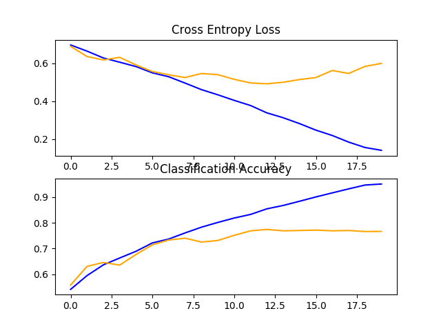

狗和猫数据集上带有两个 VGG 块的基线模型的损失和准确度学习曲线的线图

三块 VGG 模型

三块 VGG 模型扩展了两块模型并添加了具有 128 个过滤器的第三块。

该模型的define_model()函数在上一节中定义，但为了完整性在下面再次提供。

# define cnn model
def define_model():
	model = Sequential()
	model.add(Conv2D(32, (3, 3), activation='relu', kernel_initializer='he_uniform', padding='same', input_shape=(200, 200, 3)))
	model.add(MaxPooling2D((2, 2)))
	model.add(Conv2D(64, (3, 3), activation='relu', kernel_initializer='he_uniform', padding='same'))
	model.add(MaxPooling2D((2, 2)))
	model.add(Conv2D(128, (3, 3), activation='relu', kernel_initializer='he_uniform', padding='same'))
	model.add(MaxPooling2D((2, 2)))
	model.add(Flatten())
	model.add(Dense(128, activation='relu', kernel_initializer='he_uniform'))
	model.add(Dense(1, activation='sigmoid'))
	# compile model
	opt = SGD(lr=0.001, momentum=0.9)
	model.compile(optimizer=opt, loss='binary_crossentropy', metrics=['accuracy'])
	return model

运行此示例将打印训练和测试数据集的大小，确认数据集已正确加载。

对模型进行拟合和评估，并报告在测试数据集上的性能。

Found 18697 images belonging to 2 classes.
Found 6303 images belonging to 2 classes.
> 80.184

注意：你的结果可能会因算法或评估程序的随机性或数值精度的差异而有所不同。考虑多次运行该示例并比较平均结果。

在这种情况下，我们可以看到我们实现了性能的进一步提升，从使用两个块的约 76% 提高到使用三个块的约 80% 的准确率。这个结果很好，因为它接近于论文中使用 SVM 报告的现有技术水平，准确率约为 82%。

回顾学习曲线图，我们可以看到类似的过度拟合趋势，在这种情况下，可能会推迟到第 5 或第 6 个时期。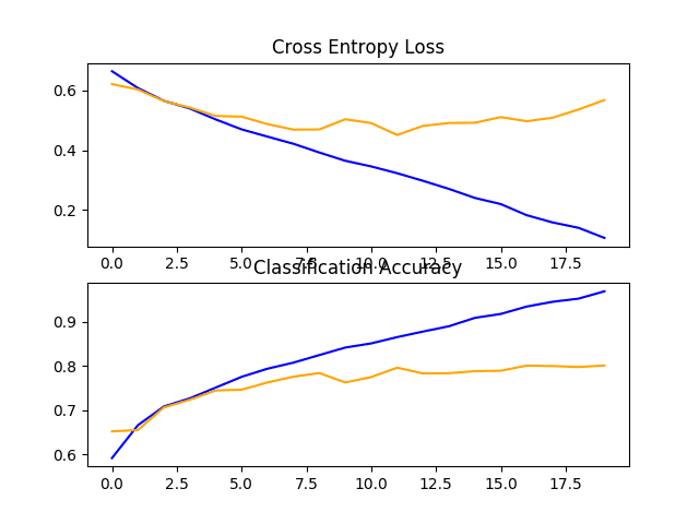

狗和猫数据集上具有三个 VGG 块的基线模型的损失和准确度学习曲线的线图

讨论

我们已经探索了基于 VGG 架构的三种不同模型。

结果可以总结如下，尽管鉴于算法的随机性，我们必须假设这些结果存在一些差异：

• VGG 1：72.331%
• VGG 2：76.646%
• VGG 3：80.184%

我们看到性能随着容量的增加而提高的趋势，但也有类似的过拟合情况在运行中越来越早发生。

结果表明该模型可能会受益于正则化技术。这可能包括诸如 dropout、权重衰减和数据增强等技术。后者还可以通过扩展训练数据集鼓励模型学习对位置进一步不变的特征来提高性能。

python识别猫狗的方法：开发模型改进

在上一节中，我们使用 VGG 样式块开发了一个基线模型，并发现了性能随着模型容量增加而提高的趋势。

在本节中，我们将从具有三个 VGG 块（即 VGG 3）的基线模型开始，并探索对该模型的一些简单改进。

从训练期间查看模型的学习曲线来看，该模型显示出强烈的过度拟合迹象。我们可以探索两种尝试解决这种过度拟合的方法：dropout 正则化和数据增强。

预计这两种方法都会减缓训练期间的改进速度，并有望对抗训练数据集的过度拟合。因此，我们将训练 epoch 的数量从 20 增加到 50，以便为模型提供更多的细化空间。

Dropout 正则化

Dropout 正则化是一种对深度神经网络进行正则化的计算成本低廉的方法。

Dropout 的工作原理是概率性地移除或“丢弃”层的输入，这些输入可能是数据样本中的输入变量或来自前一层的激活。它具有模拟大量具有非常不同网络结构的网络的效果，进而使网络中的节点通常对输入更具鲁棒性。

有关辍学的更多信息，请参阅帖子：

• 如何在 Keras 中使用 Dropout 正则化减少过拟合

通常，可以在每个 VGG 块之后应用少量的 dropout，将更多的 dropout 应用到模型输出层附近的全连接层。

下面是添加 Dropout 的基线模型更新版本的define_model()函数。在这种情况下，在每个 VGG 块之后应用 20% 的 dropout，在模型分类器部分的全连接层之后应用 50% 的较大 dropout 率。

# define cnn model
def define_model():
	model = Sequential()
	model.add(Conv2D(32, (3, 3), activation='relu', kernel_initializer='he_uniform', padding='same', input_shape=(200, 200, 3)))
	model.add(MaxPooling2D((2, 2)))
	model.add(Dropout(0.2))
	model.add(Conv2D(64, (3, 3), activation='relu', kernel_initializer='he_uniform', padding='same'))
	model.add(MaxPooling2D((2, 2)))
	model.add(Dropout(0.2))
	model.add(Conv2D(128, (3, 3), activation='relu', kernel_initializer='he_uniform', padding='same'))
	model.add(MaxPooling2D((2, 2)))
	model.add(Dropout(0.2))
	model.add(Flatten())
	model.add(Dense(128, activation='relu', kernel_initializer='he_uniform'))
	model.add(Dropout(0.5))
	model.add(Dense(1, activation='sigmoid'))
	# compile model
	opt = SGD(lr=0.001, momentum=0.9)
	model.compile(optimizer=opt, loss='binary_crossentropy', metrics=['accuracy'])
	return model

为了完整起见，下面列出了基线模型的完整代码清单，其中在狗与猫数据集上添加了 dropout。

# baseline model with dropout for the dogs vs cats dataset
import sys
from matplotlib import pyplot
from keras.utils import to_categorical
from keras.models import Sequential
from keras.layers import Conv2D
from keras.layers import MaxPooling2D
from keras.layers import Dense
from keras.layers import Flatten
from keras.layers import Dropout
from keras.optimizers import SGD
from keras.preprocessing.image import ImageDataGenerator

# define cnn model
def define_model():
	model = Sequential()
	model.add(Conv2D(32, (3, 3), activation='relu', kernel_initializer='he_uniform', padding='same', input_shape=(200, 200, 3)))
	model.add(MaxPooling2D((2, 2)))
	model.add(Dropout(0.2))
	model.add(Conv2D(64, (3, 3), activation='relu', kernel_initializer='he_uniform', padding='same'))
	model.add(MaxPooling2D((2, 2)))
	model.add(Dropout(0.2))
	model.add(Conv2D(128, (3, 3), activation='relu', kernel_initializer='he_uniform', padding='same'))
	model.add(MaxPooling2D((2, 2)))
	model.add(Dropout(0.2))
	model.add(Flatten())
	model.add(Dense(128, activation='relu', kernel_initializer='he_uniform'))
	model.add(Dropout(0.5))
	model.add(Dense(1, activation='sigmoid'))
	# compile model
	opt = SGD(lr=0.001, momentum=0.9)
	model.compile(optimizer=opt, loss='binary_crossentropy', metrics=['accuracy'])
	return model

# plot diagnostic learning curves
def summarize_diagnostics(history):
	# plot loss
	pyplot.subplot(211)
	pyplot.title('Cross Entropy Loss')
	pyplot.plot(history.history['loss'], color='blue', label='train')
	pyplot.plot(history.history['val_loss'], color='orange', label='test')
	# plot accuracy
	pyplot.subplot(212)
	pyplot.title('Classification Accuracy')
	pyplot.plot(history.history['accuracy'], color='blue', label='train')
	pyplot.plot(history.history['val_accuracy'], color='orange', label='test')
	# save plot to file
	filename = sys.argv[0].split('/')[-1]
	pyplot.savefig(filename + '_plot.png')
	pyplot.close()

# run the test harness for evaluating a model
def run_test_harness():
	# define model
	model = define_model()
	# create data generator
	datagen = ImageDataGenerator(rescale=1.0/255.0)
	# prepare iterator
	train_it = datagen.flow_from_directory('dataset_dogs_vs_cats/train/',
		class_mode='binary', batch_size=64, target_size=(200, 200))
	test_it = datagen.flow_from_directory('dataset_dogs_vs_cats/test/',
		class_mode='binary', batch_size=64, target_size=(200, 200))
	# fit model
	history = model.fit_generator(train_it, steps_per_epoch=len(train_it),
		validation_data=test_it, validation_steps=len(test_it), epochs=50, verbose=0)
	# evaluate model
	_, acc = model.evaluate_generator(test_it, steps=len(test_it), verbose=0)
	print('> %.3f' % (acc * 100.0))
	# learning curves
	summarize_diagnostics(history)

# entry point, run the test harness
run_test_harness()

运行示例首先拟合模型，然后报告模型在保持测试数据集上的性能。

注意：你的结果可能会因算法或评估程序的随机性或数值精度的差异而有所不同。考虑多次运行该示例并比较平均结果。

在这种情况下，我们可以看到模型性能从基线模型的约 80% 的准确率小幅提升到添加 dropout 的约 81%。

Found 18697 images belonging to 2 classes.
Found 6303 images belonging to 2 classes.
> 81.279

回顾学习曲线，我们可以看到 dropout 对模型在训练集和测试集上的改进率都有影响。

过度拟合已减少或延迟，但性能可能会在运行结束时开始停滞。

结果表明，进一步的训练时期可能会导致模型的进一步改进。除了训练时期的增加之外，探索 VGG 块之后的辍学率可能略高也可能很有趣。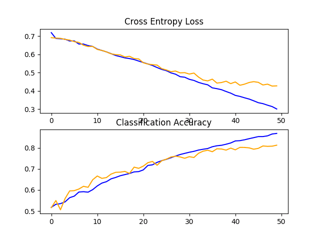

狗和猫数据集上具有 Dropout 的基线模型的损失和准确度学习曲线的线图

图像数据增强

图像数据增强是一种技术，可用于通过在数据集中创建图像的修改版本来人为地扩展训练数据集的大小。

在更多数据上训练深度学习神经网络模型可以产生更熟练的模型，而增强技术可以创建图像的变化，从而提高拟合模型将他们学到的知识推广到新图像的能力。

数据增强也可以作为一种正则化技术，为训练数据添加噪声，并鼓励模型学习相同的特征，不随它们在输入中的位置而变化。

对狗和猫的输入照片进行小幅更改可能对解决此问题有用，例如小幅移动和水平翻转。这些增强可以指定为用于训练数据集的 ImageDataGenerator 的参数。增强不应用于测试数据集，因为我们希望评估模型在未修改照片上的性能。

这要求我们有一个单独的 ImageDataGenerator 实例用于训练和测试数据集，然后是从各自的数据生成器创建的训练和测试集的迭代器。例如：

# create data generators
train_datagen = ImageDataGenerator(rescale=1.0/255.0,
	width_shift_range=0.1, height_shift_range=0.1, horizontal_flip=True)
test_datagen = ImageDataGenerator(rescale=1.0/255.0)
# prepare iterators
train_it = train_datagen.flow_from_directory('dataset_dogs_vs_cats/train/',
	class_mode='binary', batch_size=64, target_size=(200, 200))
test_it = test_datagen.flow_from_directory('dataset_dogs_vs_cats/test/',
	class_mode='binary', batch_size=64, target_size=(200, 200))

在这种情况下，训练数据集中的照片将通过小的 (10%) 随机水平和垂直移动以及随机水平翻转来增强，从而创建照片的镜像。训练和测试步骤中的照片的像素值将以相同的方式缩放。

python识别猫狗示例 - 为完整起见，下面列出了带有针对狗和猫数据集的训练数据增强的基线模型的完整代码清单。

# baseline model with data augmentation for the dogs vs cats dataset
import sys
from matplotlib import pyplot
from keras.utils import to_categorical
from keras.models import Sequential
from keras.layers import Conv2D
from keras.layers import MaxPooling2D
from keras.layers import Dense
from keras.layers import Flatten
from keras.optimizers import SGD
from keras.preprocessing.image import ImageDataGenerator

# define cnn model
def define_model():
	model = Sequential()
	model.add(Conv2D(32, (3, 3), activation='relu', kernel_initializer='he_uniform', padding='same', input_shape=(200, 200, 3)))
	model.add(MaxPooling2D((2, 2)))
	model.add(Conv2D(64, (3, 3), activation='relu', kernel_initializer='he_uniform', padding='same'))
	model.add(MaxPooling2D((2, 2)))
	model.add(Conv2D(128, (3, 3), activation='relu', kernel_initializer='he_uniform', padding='same'))
	model.add(MaxPooling2D((2, 2)))
	model.add(Flatten())
	model.add(Dense(128, activation='relu', kernel_initializer='he_uniform'))
	model.add(Dense(1, activation='sigmoid'))
	# compile model
	opt = SGD(lr=0.001, momentum=0.9)
	model.compile(optimizer=opt, loss='binary_crossentropy', metrics=['accuracy'])
	return model

# plot diagnostic learning curves
def summarize_diagnostics(history):
	# plot loss
	pyplot.subplot(211)
	pyplot.title('Cross Entropy Loss')
	pyplot.plot(history.history['loss'], color='blue', label='train')
	pyplot.plot(history.history['val_loss'], color='orange', label='test')
	# plot accuracy
	pyplot.subplot(212)
	pyplot.title('Classification Accuracy')
	pyplot.plot(history.history['accuracy'], color='blue', label='train')
	pyplot.plot(history.history['val_accuracy'], color='orange', label='test')
	# save plot to file
	filename = sys.argv[0].split('/')[-1]
	pyplot.savefig(filename + '_plot.png')
	pyplot.close()

# run the test harness for evaluating a model
def run_test_harness():
	# define model
	model = define_model()
	# create data generators
	train_datagen = ImageDataGenerator(rescale=1.0/255.0,
		width_shift_range=0.1, height_shift_range=0.1, horizontal_flip=True)
	test_datagen = ImageDataGenerator(rescale=1.0/255.0)
	# prepare iterators
	train_it = train_datagen.flow_from_directory('dataset_dogs_vs_cats/train/',
		class_mode='binary', batch_size=64, target_size=(200, 200))
	test_it = test_datagen.flow_from_directory('dataset_dogs_vs_cats/test/',
		class_mode='binary', batch_size=64, target_size=(200, 200))
	# fit model
	history = model.fit_generator(train_it, steps_per_epoch=len(train_it),
		validation_data=test_it, validation_steps=len(test_it), epochs=50, verbose=0)
	# evaluate model
	_, acc = model.evaluate_generator(test_it, steps=len(test_it), verbose=0)
	print('> %.3f' % (acc * 100.0))
	# learning curves
	summarize_diagnostics(history)

# entry point, run the test harness
run_test_harness()

运行示例首先拟合模型，然后报告模型在保持测试数据集上的性能。

注意：你的结果可能会因算法或评估程序的随机性或数值精度的差异而有所不同。考虑多次运行该示例并比较平均结果。

在这种情况下，我们可以看到性能提升了约 5%，从基线模型的约 80% 到基线模型的约 85%，通过简单的数据增强。

> 85.816

回顾学习曲线，我们可以看到模型似乎能够进一步学习，即使在运行结束时训练和测试数据集的损失仍然在减少。重复 100 个或更多 epoch 的实验很可能会产生更好的模型。

探索其他增强可能会很有趣，这些增强可能会进一步鼓励学习与其在输入中的位置不变的特征，例如小旋转和缩放。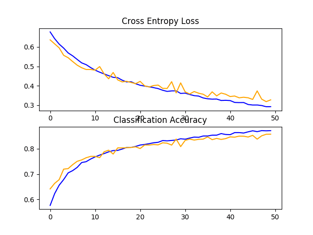

狗和猫数据集上具有数据增强的基线模型的损失和准确度学习曲线的线图

讨论

我们已经探索了对基线模型的三种不同改进。

结果可以总结如下，尽管鉴于算法的随机性，我们必须假设这些结果存在一些差异：

• 基线 VGG3 + Dropout：81.279%
• 基线 VGG3 + 数据增强：85.816

正如所怀疑的那样，正则化技术的添加减缓了学习算法的进展并减少了过度拟合，从而提高了保持数据集的性能。两种方法的结合与进一步增加训练时期的数量可能会导致进一步的改进。

这只是可以在此数据集上探索的改进类型的开始。除了对所描述的正则化方法进行调整之外，还可以探索其他正则化方法，例如权重衰减和提前停止。

可能值得探索学习算法的变化，例如学习率的变化、学习率计划的使用或自适应学习率，例如Adam。

替代模型架构也可能值得探索。所选的基线模型预计将提供比解决此问题可能需要的容量更多的容量，并且较小的模型可能会更快地训练，进而可能会产生更好的性能。

python如何识别猫狗？探索迁移学习

迁移学习涉及使用在相关任务上训练的模型的全部或部分。

Keras 提供了一系列预训练模型，可以通过Keras 应用程序 API全部或部分加载和使用这些模型。

一个有用的迁移学习模型是 VGG 模型之一，例如具有 16 层的 VGG-16，它在开发时在 ImageNet 照片分类挑战中取得了最高的成绩。

该模型由两个主要部分组成，模型的特征提取器部分由 VGG 块组成，模型的分类器部分由全连接层和输出层组成。

我们可以使用模型的特征提取部分，并添加模型的新分类器部分，该部分是针对狗和猫数据集量身定制的。具体来说，我们可以在训练期间保持所有卷积层的权重固定，并且只训练新的全连接层，这些层将学习解释从模型中提取的特征并进行二元分类。

这可以通过加载VGG-16 模型，从模型的输出端移除全连接层，然后添加新的全连接层来解释模型输出并进行预测来实现。模型的分类器部分可以通过将“ include_top ”参数设置为“ False ”来自动删除，这也要求也为模型指定输入的形状，在这种情况下为 (224, 224, 3)。这意味着加载的模型在最后一个最大池化层结束，之后我们可以手动添加一个Flatten层和新的分类器层。

下面的define_model()函数实现了这一点，并返回一个准备好训练的新模型。

# define cnn model
def define_model():
	# load model
	model = VGG16(include_top=False, input_shape=(224, 224, 3))
	# mark loaded layers as not trainable
	for layer in model.layers:
		layer.trainable = False
	# add new classifier layers
	flat1 = Flatten()(model.layers[-1].output)
	class1 = Dense(128, activation='relu', kernel_initializer='he_uniform')(flat1)
	output = Dense(1, activation='sigmoid')(class1)
	# define new model
	model = Model(inputs=model.inputs, outputs=output)
	# compile model
	opt = SGD(lr=0.001, momentum=0.9)
	model.compile(optimizer=opt, loss='binary_crossentropy', metrics=['accuracy'])
	return model

创建后，我们可以像以前一样在训练数据集上训练模型。

在这种情况下不需要大量训练，因为只有新的全连接层和输出层具有可训练的权重。因此，我们将训练 epoch 的数量固定为 10。

VGG16 模型是在特定的 ImageNet 挑战数据集上训练的。因此，它被配置为预期输入图像具有 224×224 像素的形状。当从狗和猫数据集加载照片时，我们将使用它作为目标尺寸。

该模型还希望图像居中。也就是说，从输入中减去在 ImageNet 训练数据集上计算的每个通道（红色、绿色和蓝色）的平均像素值。Keras 提供了一个函数来通过preprocess_input()函数为单张照片执行此准备工作。尽管如此，我们可以通过将“ featurewise_center ”参数设置为“ True ”并手动指定在居中时使用的平均像素值作为 ImageNet 训练数据集的平均值来使用ImageDataGenerator 实现相同的效果：[123.68, 116.779, 103.939] .

python识别猫狗示例：下面列出了在狗与猫数据集上进行迁移学习的 VGG 模型的完整代码清单。

# vgg16 model used for transfer learning on the dogs and cats dataset
import sys
from matplotlib import pyplot
from keras.utils import to_categorical
from keras.applications.vgg16 import VGG16
from keras.models import Model
from keras.layers import Dense
from keras.layers import Flatten
from keras.optimizers import SGD
from keras.preprocessing.image import ImageDataGenerator

# define cnn model
def define_model():
	# load model
	model = VGG16(include_top=False, input_shape=(224, 224, 3))
	# mark loaded layers as not trainable
	for layer in model.layers:
		layer.trainable = False
	# add new classifier layers
	flat1 = Flatten()(model.layers[-1].output)
	class1 = Dense(128, activation='relu', kernel_initializer='he_uniform')(flat1)
	output = Dense(1, activation='sigmoid')(class1)
	# define new model
	model = Model(inputs=model.inputs, outputs=output)
	# compile model
	opt = SGD(lr=0.001, momentum=0.9)
	model.compile(optimizer=opt, loss='binary_crossentropy', metrics=['accuracy'])
	return model

# plot diagnostic learning curves
def summarize_diagnostics(history):
	# plot loss
	pyplot.subplot(211)
	pyplot.title('Cross Entropy Loss')
	pyplot.plot(history.history['loss'], color='blue', label='train')
	pyplot.plot(history.history['val_loss'], color='orange', label='test')
	# plot accuracy
	pyplot.subplot(212)
	pyplot.title('Classification Accuracy')
	pyplot.plot(history.history['accuracy'], color='blue', label='train')
	pyplot.plot(history.history['val_accuracy'], color='orange', label='test')
	# save plot to file
	filename = sys.argv[0].split('/')[-1]
	pyplot.savefig(filename + '_plot.png')
	pyplot.close()

# run the test harness for evaluating a model
def run_test_harness():
	# define model
	model = define_model()
	# create data generator
	datagen = ImageDataGenerator(featurewise_center=True)
	# specify imagenet mean values for centering
	datagen.mean = [123.68, 116.779, 103.939]
	# prepare iterator
	train_it = datagen.flow_from_directory('dataset_dogs_vs_cats/train/',
		class_mode='binary', batch_size=64, target_size=(224, 224))
	test_it = datagen.flow_from_directory('dataset_dogs_vs_cats/test/',
		class_mode='binary', batch_size=64, target_size=(224, 224))
	# fit model
	history = model.fit_generator(train_it, steps_per_epoch=len(train_it),
		validation_data=test_it, validation_steps=len(test_it), epochs=10, verbose=1)
	# evaluate model
	_, acc = model.evaluate_generator(test_it, steps=len(test_it), verbose=0)
	print('> %.3f' % (acc * 100.0))
	# learning curves
	summarize_diagnostics(history)

# entry point, run the test harness
run_test_harness()

运行示例首先拟合模型，然后报告模型在保持测试数据集上的性能。

注意：你的结果可能会因算法或评估程序的随机性或数值精度的差异而有所不同。考虑多次运行该示例并比较平均结果。

在这种情况下，我们可以看到该模型在保持测试数据集上取得了令人印象深刻的结果，分类准确率约为 97%。

Found 18697 images belonging to 2 classes.
Found 6303 images belonging to 2 classes.
> 97.636

查看学习曲线，我们可以看到模型快速拟合数据集。它没有表现出强烈的过度拟合，尽管结果表明分类器中的额外容量和/或正则化的使用可能会有所帮助。

这种方法可以进行许多改进，包括向模型的分类器部分添加 dropout 正则化，甚至可能微调模型的特征检测器部分中部分或全部层的权重。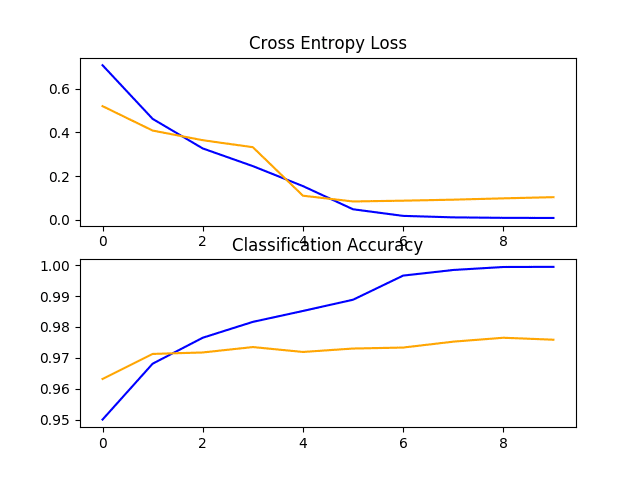

狗和猫数据集上 VGG16 迁移学习模型的损失和准确度学习曲线的线图

如何完成模型并进行预测

只要我们有想法、有时间和资源来测试它们，模型改进的过程就可能会持续下去。

在某些时候，必须选择并采用最终的模型配置。在这种情况下，我们将保持简单并使用 VGG-16 迁移学习方法作为最终模型。

首先，我们将通过在整个训练数据集上拟合模型并将模型保存到文件以供以后使用来最终确定我们的模型。然后我们将加载保存的模型并使用它对单个图像进行预测。

对狗和猫的照片进行分类：准备最终数据集

最终模型通常适用于所有可用数据，例如所有训练和测试数据集的组合。

在本教程中，我们将演示仅在训练数据集上拟合的最终模型，因为我们只有训练数据集的标签。

第一步是准备训练数据集，以便ImageDataGenerator类可以通过flow_from_directory()函数加载它。具体来说，我们需要创建一个新目录，将所有训练图像组织到dog/和cats/子目录中，而没有任何分离到train/或test/目录。

这可以通过更新我们在教程开头开发的脚本来实现。在这种情况下，我们将为整个训练数据集创建一个新的finalize_dogs_vs_cats/文件夹，其中包含dogs/和cats/子文件夹。

结构如下：

finalize_dogs_vs_cats
├── cats
└── dogs

为了完整起见，下面列出了更新的脚本。

# organize dataset into a useful structure
from os import makedirs
from os import listdir
from shutil import copyfile
# create directories
dataset_home = 'finalize_dogs_vs_cats/'
# create label subdirectories
labeldirs = ['dogs/', 'cats/']
for labldir in labeldirs:
	newdir = dataset_home + labldir
	makedirs(newdir, exist_ok=True)
# copy training dataset images into subdirectories
src_directory = 'dogs-vs-cats/train/'
for file in listdir(src_directory):
	src = src_directory + '/' + file
	if file.startswith('cat'):
		dst = dataset_home + 'cats/'  + file
		copyfile(src, dst)
	elif file.startswith('dog'):
		dst = dataset_home + 'dogs/'  + file
		copyfile(src, dst)

保存最终模型

python如何识别猫狗？我们现在准备在整个训练数据集上拟合最终模型。

该flow_from_directory（）必须更新加载的所有图像从新finalize_dogs_vs_cats /目录。

# prepare iterator
train_it = datagen.flow_from_directory('finalize_dogs_vs_cats/',
	class_mode='binary', batch_size=64, target_size=(224, 224))

此外，对fit_generator()的调用不再需要指定验证数据集。

# fit model
model.fit_generator(train_it, steps_per_epoch=len(train_it), epochs=10, verbose=0)

拟合后，我们可以通过调用模型上的save()函数并传入所选文件名，将最终模型保存到 H5 文件中。

# save model
model.save('final_model.h5')

请注意，保存和加载Keras模型需要在你的工作站上安装h5py 库。

下面列出了在训练数据集上拟合最终模型并将其保存到文件的完整python识别猫狗示例。

# save the final model to file
from keras.applications.vgg16 import VGG16
from keras.models import Model
from keras.layers import Dense
from keras.layers import Flatten
from keras.optimizers import SGD
from keras.preprocessing.image import ImageDataGenerator

# define cnn model
def define_model():
	# load model
	model = VGG16(include_top=False, input_shape=(224, 224, 3))
	# mark loaded layers as not trainable
	for layer in model.layers:
		layer.trainable = False
	# add new classifier layers
	flat1 = Flatten()(model.layers[-1].output)
	class1 = Dense(128, activation='relu', kernel_initializer='he_uniform')(flat1)
	output = Dense(1, activation='sigmoid')(class1)
	# define new model
	model = Model(inputs=model.inputs, outputs=output)
	# compile model
	opt = SGD(lr=0.001, momentum=0.9)
	model.compile(optimizer=opt, loss='binary_crossentropy', metrics=['accuracy'])
	return model

# run the test harness for evaluating a model
def run_test_harness():
# define model
	model = define_model()
	# create data generator
	datagen = ImageDataGenerator(featurewise_center=True)
	# specify imagenet mean values for centering
	datagen.mean = [123.68, 116.779, 103.939]
	# prepare iterator
	train_it = datagen.flow_from_directory('finalize_dogs_vs_cats/',
		class_mode='binary', batch_size=64, target_size=(224, 224))
	# fit model
	model.fit_generator(train_it, steps_per_epoch=len(train_it), epochs=10, verbose=0)
	# save model
	model.save('final_model.h5')

# entry point, run the test harness
run_test_harness()

运行此示例后，你现在将在当前工作目录中拥有一个名为“ final_model.h5 ”的81 兆字节大文件。

做预测

我们可以使用我们保存的模型对新图像进行预测。

该模型假设新图像是彩色的，并且它们已被分割，因此一张图像至少包含一只狗或猫。

下面是从狗和猫比赛的测试数据集中提取的图像。它没有标签，但我们可以清楚地看出这是一张狗的照片。你可以使用文件名“ sample_image.jpg ”将其保存在当前工作目录中。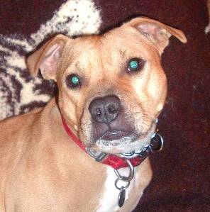

狗 (sample_image.jpg)

• 下载狗照片 (sample_image.jpg)

我们将假装这是一张全新的、看不见的图像，以所需的方式准备，看看我们如何使用我们保存的模型来预测图像代表的整数。对于这个例子，我们期望“ Dog ”的类“ 1 ”。

注意：图像的子目录，每个类一个，由flow_from_directory()函数按字母顺序加载，并为每个类分配一个整数。子目录“ cat ”出现在“ dog ”之前，因此类标签被分配了整数：cat=0, dog=1。这可以通过在训练模型时调用flow_from_directory() 中的“ classes ”参数进行更改。

python如何识别猫狗？首先，我们可以加载图像并强制其大小为 224×224 像素。然后可以调整加载的图像的大小以在数据集中包含单个样本。像素值还必须居中以匹配模型训练期间准备数据的方式。该load_image（）函数实现这一点，将返回加载图像准备进行分类。

# load and prepare the image
def load_image(filename):
	# load the image
	img = load_img(filename, target_size=(224, 224))
	# convert to array
	img = img_to_array(img)
	# reshape into a single sample with 3 channels
	img = img.reshape(1, 224, 224, 3)
	# center pixel data
	img = img.astype('float32')
	img = img - [123.68, 116.779, 103.939]
	return img

接下来，我们可以像上一节一样加载模型并调用 predict() 函数将图像中的内容分别预测为“ cat ”和“ dog ”的“ 0 ”和“ 1 ”之间的数字。

# predict the class
result = model.predict(img)

下面列出了完整的python识别猫狗示例。

# make a prediction for a new image.
from keras.preprocessing.image import load_img
from keras.preprocessing.image import img_to_array
from keras.models import load_model

# load and prepare the image
def load_image(filename):
	# load the image
	img = load_img(filename, target_size=(224, 224))
	# convert to array
	img = img_to_array(img)
	# reshape into a single sample with 3 channels
	img = img.reshape(1, 224, 224, 3)
	# center pixel data
	img = img.astype('float32')
	img = img - [123.68, 116.779, 103.939]
	return img

# load an image and predict the class
def run_example():
	# load the image
	img = load_image('sample_image.jpg')
	# load model
	model = load_model('final_model.h5')
	# predict the class
	result = model.predict(img)
	print(result[0])

# entry point, run the example
run_example()

运行示例首先加载并准备图像，加载模型，然后正确预测加载的图像代表“狗”或“ 1 ”类。

1

扩展

python识别猫狗的方法 - 本节列出了你可能希望探索的扩展教程的一些想法。

• 调整正则化。探索在基线模型上使用的正则化技术的细微变化，例如不同的丢失率和不同的图像增强。
• 调整学习率。探索用于训练基线模型的学习算法的变化，例如替代学习率、学习率计划或自适应学习率算法（如 Adam）。
• 备用预训练模型。探索用于该问题的迁移学习的替代预训练模型，例如 Inception 或 ResNet。

如果你探索这些扩展中的任何一个，我很想知道。
在下面的评论中发布你的发现。

进一步阅读

如果你想深入了解，本节将提供有关该主题的更多资源。

文件

• Asirra：利用兴趣对齐的手动图像分类的 CAPTCHA，2007 年。
• 针对 Asirra CAPTCHA 的机器学习攻击，2007 年。
• OverFeat：使用卷积网络的集成识别、定位和检测，2013 年。

应用程序接口

• Keras 应用程序 API
• Keras 图像处理 API
• Keras 顺序模型 API

文章

• 狗 vs 猫 Kaggle 比赛。
• Dogs vs. Cats Redux：内核版。
• 狗 vs 猫数据集，Kaggle。
• 使用很少的数据构建强大的图像分类模型，2016 年。

概括

python如何识别猫狗？在本教程中，你了解了如何开发卷积神经网络来对狗和猫的照片进行分类。

具体来说，你学到了：

• 如何加载和准备用于建模的狗和猫的照片。
• 如何从头开发用于照片分类的卷积神经网络并提高模型性能。
• 如何使用迁移学习开发照片分类模型。

你有任何问题吗？
在下面的评论中提出你的问题，我会尽力回答。