在本Python逻辑回归教程中,我将向你展示 Python 中的 Logistic 回归示例。
一般而言,二元逻辑回归描述因二元变量与一个或多个自变量之间的关系。
二元因变量有两种可能的结果:
- '1' 表示true/成功;或者
- '0' 表示false/失败
现在让我们通过一个实际Python逻辑回归示例来看看如何在 Python 中应用逻辑回归。
在 Python 中应用逻辑回归的步骤
第 1 步:收集数据
Python如何实现逻辑回归?首先举一个简单的例子,假设你的目标是用 Python 构建逻辑回归模型,以确定候选人是否会被名牌大学录取。
在这里,有两种可能的结果:Admitted(由“1”的值表示)与被拒绝Rejected(由“0”的值表示)。
然后,你可以在 Python 中构建逻辑回归,其中:
- 因变量表示一个人是否被录取;和
- 3 个自变量是 GMAT 分数、GPA 和工作经验年数
这是数据集的样子:
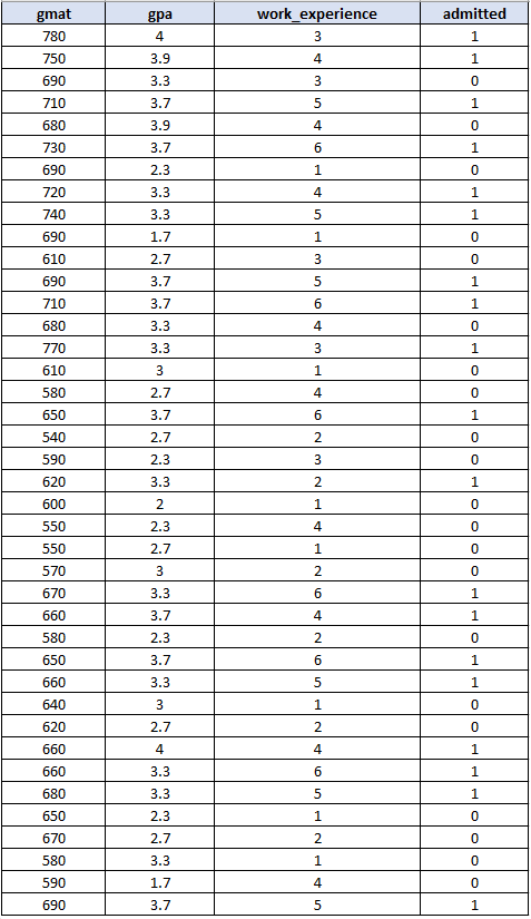
请注意,上述数据集包含 40 个观察值。实际上,你需要更大的样本量才能获得更准确的结果。
第 2 步:导入所需的 Python 包
在开始之前,请确保在 Python中安装了以下软件包:
- pandas – 用于创建 DataFrame 以在 Python 中捕获数据集
- sklearn – 用于在 Python 中构建逻辑回归模型
- seaborn – 用于创建混淆矩阵
- matplotlib – 用于显示图表
然后,你需要按如下方式导入所有包:
import pandas as pd
from sklearn.model_selection import train_test_split
from sklearn.linear_model import LogisticRegression
from sklearn import metrics
import seaborn as sn
import matplotlib.pyplot as plt
第 3 步:构建dataframe
对于此步骤,你需要在 Python 中捕获数据集(来自步骤 1)。你可以使用pandas Dataframe完成此任务,如下Python逻辑回归代码示例:
import pandas as pd
candidates = {'gmat': [780,750,690,710,680,730,690,720,740,690,610,690,710,680,770,610,580,650,540,590,620,600,550,550,570,670,660,580,650,660,640,620,660,660,680,650,670,580,590,690],
              'gpa': [4,3.9,3.3,3.7,3.9,3.7,2.3,3.3,3.3,1.7,2.7,3.7,3.7,3.3,3.3,3,2.7,3.7,2.7,2.3,3.3,2,2.3,2.7,3,3.3,3.7,2.3,3.7,3.3,3,2.7,4,3.3,3.3,2.3,2.7,3.3,1.7,3.7],
              'work_experience': [3,4,3,5,4,6,1,4,5,1,3,5,6,4,3,1,4,6,2,3,2,1,4,1,2,6,4,2,6,5,1,2,4,6,5,1,2,1,4,5],
              'admitted': [1,1,0,1,0,1,0,1,1,0,0,1,1,0,1,0,0,1,0,0,1,0,0,0,0,1,1,0,1,1,0,0,1,1,1,0,0,0,0,1]
              }

df = pd.DataFrame(candidates,columns= ['gmat', 'gpa','work_experience','admitted'])
print (df)
或者,你可以将数据从外部文件导入 Python。
第 4 步:在 Python 中创建逻辑回归
Python逻辑回归示例:现在,设置自变量(表示为 X)和因变量(表示为 y):
X = df[['gmat', 'gpa','work_experience']]
y = df['admitted']然后,应用train_test_split。例如,你可以将测试大小设置为0.25,因此模型测试将基于数据集的 25%,而模型训练将基于数据集的 75%:
X_train,X_test,y_train,y_test = train_test_split(X,y,test_size=0.25,random_state=0)应用逻辑回归如下:
logistic_regression= LogisticRegression()
logistic_regression.fit(X_train,y_train)
y_pred=logistic_regression.predict(X_test)
然后,使用下面的代码来获取混淆矩阵:
confusion_matrix = pd.crosstab(y_test, y_pred, rownames=['Actual'], colnames=['Predicted'])
sn.heatmap(confusion_matrix, annot=True)
Python逻辑回归教程:对于最后一部分,打印精度并绘制混淆矩阵:
print('Accuracy: ',metrics.accuracy_score(y_test, y_pred))
plt.show()将所有代码组件放在一起,如下是完整的Python逻辑回归代码示例:
import pandas as pd
from sklearn.model_selection import train_test_split
from sklearn.linear_model import LogisticRegression
from sklearn import metrics
import seaborn as sn
import matplotlib.pyplot as plt

candidates = {'gmat': [780,750,690,710,680,730,690,720,740,690,610,690,710,680,770,610,580,650,540,590,620,600,550,550,570,670,660,580,650,660,640,620,660,660,680,650,670,580,590,690],
              'gpa': [4,3.9,3.3,3.7,3.9,3.7,2.3,3.3,3.3,1.7,2.7,3.7,3.7,3.3,3.3,3,2.7,3.7,2.7,2.3,3.3,2,2.3,2.7,3,3.3,3.7,2.3,3.7,3.3,3,2.7,4,3.3,3.3,2.3,2.7,3.3,1.7,3.7],
              'work_experience': [3,4,3,5,4,6,1,4,5,1,3,5,6,4,3,1,4,6,2,3,2,1,4,1,2,6,4,2,6,5,1,2,4,6,5,1,2,1,4,5],
              'admitted': [1,1,0,1,0,1,0,1,1,0,0,1,1,0,1,0,0,1,0,0,1,0,0,0,0,1,1,0,1,1,0,0,1,1,1,0,0,0,0,1]
              }

df = pd.DataFrame(candidates,columns= ['gmat', 'gpa','work_experience','admitted'])

#print (df)

X = df[['gmat', 'gpa','work_experience']]
y = df['admitted']

X_train,X_test,y_train,y_test = train_test_split(X,y,test_size=0.25,random_state=0)

logistic_regression= LogisticRegression()
logistic_regression.fit(X_train,y_train)
y_pred=logistic_regression.predict(X_test)

confusion_matrix = pd.crosstab(y_test, y_pred, rownames=['Actual'], colnames=['Predicted'])
sn.heatmap(confusion_matrix, annot=True)

print('Accuracy: ',metrics.accuracy_score(y_test, y_pred))
plt.show()
在 Python 中运行代码,你将获得以下准确度为0.8 的混淆矩阵(请注意,根据你的 sklearn 版本,你可能会得到不同的准确度结果。在我的情况下,sklearn 版本为 0.22.2):
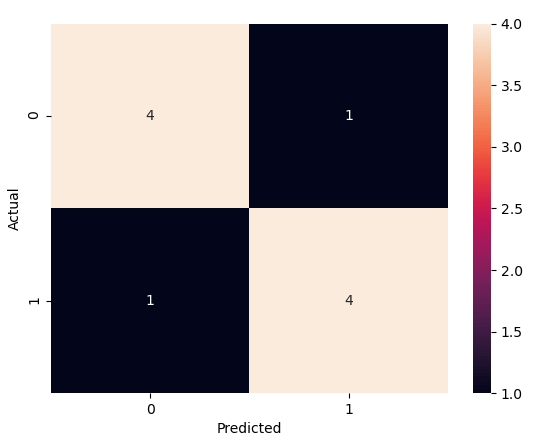
从矩阵可以看出:
- TP = True Positives = 4
- TN = True Negatives = 4
- FP = False Positives = 1
- FN = False Negatives = 1
然后,你还可以 使用以下方法获得准确度:
准确率 = (TP+TN)/总= (4+4)/10 = 0.8
因此,测试集的准确度为 80%。
Python如何实现逻辑回归?深入研究结果
现在让我们在 python 代码中打印两个组件:
- print(X_test)
- print(y_pred)
这是使用的Python逻辑回归代码示例:
import pandas as pd
from sklearn.model_selection import train_test_split
from sklearn.linear_model import LogisticRegression

candidates = {'gmat': [780,750,690,710,680,730,690,720,740,690,610,690,710,680,770,610,580,650,540,590,620,600,550,550,570,670,660,580,650,660,640,620,660,660,680,650,670,580,590,690],
              'gpa': [4,3.9,3.3,3.7,3.9,3.7,2.3,3.3,3.3,1.7,2.7,3.7,3.7,3.3,3.3,3,2.7,3.7,2.7,2.3,3.3,2,2.3,2.7,3,3.3,3.7,2.3,3.7,3.3,3,2.7,4,3.3,3.3,2.3,2.7,3.3,1.7,3.7],
              'work_experience': [3,4,3,5,4,6,1,4,5,1,3,5,6,4,3,1,4,6,2,3,2,1,4,1,2,6,4,2,6,5,1,2,4,6,5,1,2,1,4,5],
              'admitted': [1,1,0,1,0,1,0,1,1,0,0,1,1,0,1,0,0,1,0,0,1,0,0,0,0,1,1,0,1,1,0,0,1,1,1,0,0,0,0,1]
              }

df = pd.DataFrame(candidates,columns= ['gmat', 'gpa','work_experience','admitted'])

X = df[['gmat', 'gpa','work_experience']]
y = df['admitted']

X_train,X_test,y_train,y_test = train_test_split(X,y,test_size=0.25,random_state=0)  #train is based on 75% of the dataset, test is based on 25% of dataset

logistic_regression= LogisticRegression()
logistic_regression.fit(X_train,y_train)
y_pred=logistic_regression.predict(X_test)

print (X_test) #test dataset
print (y_pred) #predicted values
回想一下我们的原始数据集(来自步骤 1)有 40 个观察值。由于我们将测试大小设置为 0.25,因此混淆矩阵显示了 10 条记录(=40*0.25)的结果。这些是 10 个测试记录:
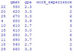
还对这 10 条记录进行了预测(其中 1 = 被录取,而 0 = 被拒绝):

在实际数据集(来自第 1 步)中,你会看到对于测试数据,我们得到了 10 次中有 8 次正确的结果:
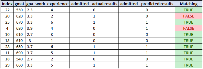
这与 80% 的准确率匹配
检查新数据集的预测
Python逻辑回归示例:假设你有一组新数据,其中有 5 个新候选项:
| gmat | gpa | work_experience |
| 590 | 2 | 3 |
| 740 | 3.7 | 4 |
| 680 | 3.3 | 6 |
| 610 | 2.3 | 1 |
| 710 | 3 | 5 |
Python如何实现逻辑回归?你的目标是使用现有的逻辑回归模型来预测新候选人是否会被录取。
然后可以在名为df2的第二个 DataFrame 中捕获新的数据集:
new_candidates = {'gmat': [590,740,680,610,710],
                  'gpa': [2,3.7,3.3,2.3,3],
                  'work_experience': [3,4,6,1,5]
                  }

df2 = pd.DataFrame(new_candidates,columns= ['gmat', 'gpa','work_experience'])
这是获得 5 个新候选者预测的Python逻辑回归代码示例:
import pandas as pd
from sklearn.model_selection import train_test_split
from sklearn.linear_model import LogisticRegression

candidates = {'gmat': [780,750,690,710,680,730,690,720,740,690,610,690,710,680,770,610,580,650,540,590,620,600,550,550,570,670,660,580,650,660,640,620,660,660,680,650,670,580,590,690],
              'gpa': [4,3.9,3.3,3.7,3.9,3.7,2.3,3.3,3.3,1.7,2.7,3.7,3.7,3.3,3.3,3,2.7,3.7,2.7,2.3,3.3,2,2.3,2.7,3,3.3,3.7,2.3,3.7,3.3,3,2.7,4,3.3,3.3,2.3,2.7,3.3,1.7,3.7],
              'work_experience': [3,4,3,5,4,6,1,4,5,1,3,5,6,4,3,1,4,6,2,3,2,1,4,1,2,6,4,2,6,5,1,2,4,6,5,1,2,1,4,5],
              'admitted': [1,1,0,1,0,1,0,1,1,0,0,1,1,0,1,0,0,1,0,0,1,0,0,0,0,1,1,0,1,1,0,0,1,1,1,0,0,0,0,1]
              }

df = pd.DataFrame(candidates,columns= ['gmat', 'gpa','work_experience','admitted'])


X = df[['gmat', 'gpa','work_experience']]
y = df['admitted']

X_train,X_test,y_train,y_test = train_test_split(X,y,test_size=0.25,random_state=0)  #in this case, you may choose to set the test_size=0. You should get the same prediction here

logistic_regression= LogisticRegression()
logistic_regression.fit(X_train,y_train)


new_candidates = {'gmat': [590,740,680,610,710],
                  'gpa': [2,3.7,3.3,2.3,3],
                  'work_experience': [3,4,6,1,5]
                  }

df2 = pd.DataFrame(new_candidates,columns= ['gmat', 'gpa','work_experience'])
y_pred=logistic_regression.predict(df2)

print (df2)
print (y_pred)
运行代码,你会得到以下预测:
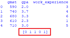
预计第一和第四名候选人不会被录取,而其他候选人预计会被录取。
以上就是Python逻辑回归示例的全部内容,希望可以帮助到你,若有问题,请在下方评论,谢谢阅读。