R编程中的回归及其类型

回归分析是一种估算两个或多个变量之间关系的统计工具。总会有一个响应变量和一个或多个预测变量。回归分析被广泛用于相应地拟合数据, 并进一步预测数据以进行预测。它可以帮助企业和组织使用因变量/响应变量和自变量/预测变量来了解其产品在市场中的行为。在本文中, 让我们了解不同类型的回归R编程借助示例。

回归类型

R编程中主要有三种类型的回归被广泛使用。他们是：

1. 线性回归
2. 多重回归
3. 逻辑回归

线性回归

线性回归模型是三种回归类型中广泛使用的模型之一。在线性回归中, 估计两个变量之间的关系, 即一个响应变量和一个预测变量。线性回归在图形上产生一条直线。数学上

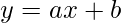
其中, x表示预测变量或自变量y表示响应变量或因变量a和b为系数

在R中实施

在R程式设计中lm()函数用于创建线性回归模型。

语法：lm(公式)参数：公式：表示必须在其上拟合数据的公式要了解更多可选参数, 请在控制台中使用以下命令：help(" lm")

例子：

在此示例中, 让我们在图形上绘制线性回归线, 并根据身高预测体重。

# R program to illustrate
# Linear Regression
  
# Height vector
x <- c (153, 169, 140, 186, 128, 136, 178, 163, 152, 133)
  
# Weight vector
y <- c (64, 81, 58, 91, 47, 57, 75, 72, 62, 49)
  
# Create a linear regression model
model <- lm (y~x)
  
# Print regression model
print (model)
  
# Find the weight of a person 
# With height 182
df <- data.frame (x = 182)
res <-  predict (model, df)
cat ("\nPredicted value of a person 
                with height = 182")
print (res)
  
# Output to be present as PNG file
png (file = "linearRegGFG.png" )
  
# Plot
plot (x, y, main = "Height vs Weight
                  Regression model")
abline ( lm (y~x))
  
# Save the file.
dev.off ()

输出如下：

Call:
lm(formula = y ~ x)

Coefficients:
(Intercept)            x  
   -39.7137       0.6847

Predicted value of a person with height = 182
      1 
84.9098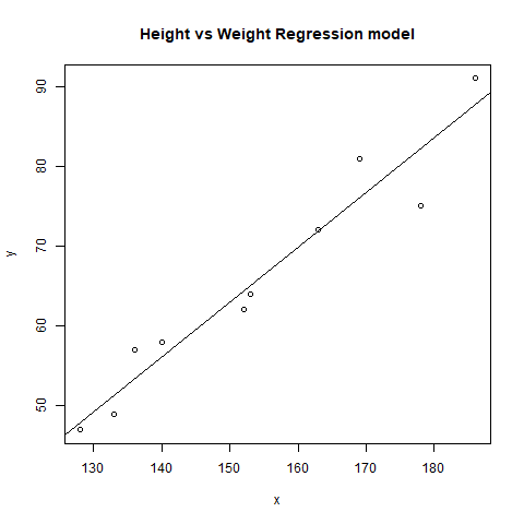

多重回归

多元回归是回归分析技术的另一种类型, 它是线性回归模型的扩展, 因为它使用多个预测变量来创建模型。数学上

在R中实施

R编程中的多元回归使用相同的lm()函数来创建模型。

语法：lm(公式, 数据)参数：公式：表示必须在其上拟合数据的公式数据：表示必须在其上应用公式的数据框

例子：

让我们创建R基础包中存在的空气质量数据集的多元回归模型, 并将该模型绘制在图上。

# R program to illustrate
# Multiple Linear Regression
  
# Using airquality dataset
input <- airquality[1:50, c ( "Ozone" , "Wind" , "Temp" )]
  
# Create regression model
model <- lm (Ozone~Wind + Temp, data = input)
  
# Print the regression model
cat ( "Regression model:\n" )
print (model)
  
# Output to be present as PNG file
png (file = "multipleRegGFG.png" )
  
# Plot
plot (model)
  
# Save the file.
dev.off ()

输出如下：

Regression model:
Call:
lm(formula = Ozone ~ Wind + Temp, data = input)

Coefficients:
(Intercept)         Wind         Temp  
    -58.239       -0.739        1.329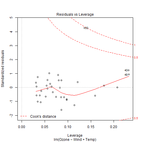

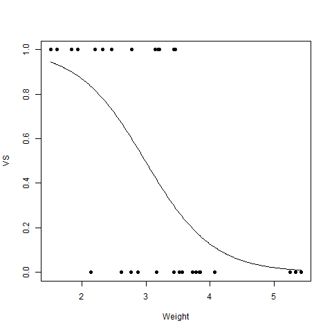
逻辑回归

Logistic回归是另一种广泛使用的回归分析技术, 可预测范围内的值。此外, 它用于预测分类数据的值。例如, 电子邮件既可以是垃圾邮件, 也可以是非垃圾邮件, 无论是赢家还是输家, 无论是男性还是女性, 等等。

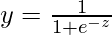
其中, y表示响应变量z表示自变量或特征的方程

在R中实施

在R程式设计中glm()函数用于创建逻辑回归模型。

语法：glm(公式, 数据, 族)参数：公式：代表必须根据其拟合模型的公式数据：代表必须在其上应用公式的数据框家族：代表要使用的功能类型。 Logistic回归的"二项式"

例子：

# R program to illustrate
# Logistic Regression
  
# Using mtcars dataset 
# To create the logistic model
model <- glm (formula = vs ~ wt, family = binomial, data = mtcars)
  
# Creating a range of wt values
x <- seq ( min (mtcars$wt), max (mtcars$wt), 0.01)
  
# Predict using weight
y <- predict (model, list (wt = x), type = "response" )
  
# Print model
print (model)
  
# Output to be present as PNG file
png (file = "LogRegGFG.png" )
  
# Plot
plot (mtcars$wt, mtcars$vs, pch = 16, xlab = "Weight" , ylab = "VS" )
lines (x, y)
  
# Saving the file
dev.off ()

输出如下：

Call:  glm(formula = vs ~ wt, family = binomial, data = mtcars)

Coefficients:
(Intercept)           wt  
      5.715       -1.911  

Degrees of Freedom: 31 Total (i.e. Null);  30 Residual
Null Deviance:      43.86 
Residual Deviance: 31.37        AIC: 35.37

---