在机器学习中, 梯度下降是一种用于计算模型参数(系数和偏差)的优化技术, 用于线性回归, 对数回归, 神经网络等算法。在此技术中, 我们反复遍历训练集并更新模型相对于训练集的误差梯度的参数。
根据更新模型参数时考虑的训练示例数量, 我们有3种类型的梯度下降:
| 批次梯度下降 | 随机梯度下降 | 小批量梯度下降 |
| 由于在迈向梯度方向之前要考虑整个训练数据, 因此进行单个更新会花费大量时间。 | 由于在朝梯度方向迈进之前仅考虑了一个训练示例, 因此我们被迫遍历训练集, 因此无法利用与代码矢量化相关的速度。 | 由于考虑了训练示例的子集, 因此它可以快速更新模型参数, 还可以利用与代码矢量化相关的速度。 |
| 可以平滑更新模型参数 | 它在参数中进行非常嘈杂的更新 | 根据批次的大小, 可以使更新的噪声更少–批次大小越大, 更新的噪声就越小 |
因此, 小批量梯度下降在快速收敛和与梯度更新相关的噪声之间做出了折衷, 这使其成为一种更加灵活和健壮的算法。
小批量梯度下降:
算法-
令theta =模型参数, max_iters =时期数。 for itr = 1, 2, 3, …, max_iters:对于mini_batch(X_mini, y_mini):在批处理X_mini上进行正向传递:对mini-batch的预测进行预测(J(theta)), 当前值为参数Backward Pass:计算梯度θ=Jθwrt的偏导数theta更新参数:theta = theta – learning_rate * gradient(theta)
以下是Python实现:
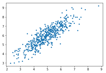
第1步:第一步是导入依赖关系, 生成用于线性回归的数据并可视化生成的数据。我们已经生成了8000个数据示例, 每个示例都有2个属性/功能。这些数据示例进一步分为训练集(X_train, y_train)和测试集(X_test, y_test), 分别具有7200和800个示例。
# importing dependencies
import numpy as np
import matplotlib.pyplot as plt

# creating data
mean = np.array([ 5.0 , 6.0 ])
cov = np.array([[ 1.0 , 0.95 ], [ 0.95 , 1.2 ]])
data = np.random.multivariate_normal(mean, cov, 8000 )

# visualising data
plt.scatter(data[: 500 , 0 ], data[: 500 , 1 ], marker = '.' )
plt.show()

# train-test-split
data = np.hstack((np.ones((data.shape[ 0 ], 1 )), data))

split_factor = 0.90
split = int (split_factor * data.shape[ 0 ])

X_train = data[:split, : - 1 ]
y_train = data[:split, - 1 ].reshape(( - 1 , 1 ))
X_test = data[split:, : - 1 ]
y_test = data[split:, - 1 ].reshape(( - 1 , 1 ))

print ( "Number of examples in training set = % d" % (X_train.shape[ 0 ]))
print ( "Number of examples in testing set = % d" % (X_test.shape[ 0 ]))
输出如下:
训练集中的示例数= 7200
测试集中的示例数= 800
第2步:
接下来, 我们编写使用最小批量梯度下降实现线性回归的代码。
梯度下降()
是主要的驱动程序功能, 其他功能是用于进行预测的辅助功能–
假设()
, 计算渐变–
梯度()
, 计算错误–
成本()
并创建小批量–
create_mini_batches()
。驱动程序函数初始化参数, 为模型计算最佳的参数集, 然后返回这些参数以及包含错误历史记录的列表, 这些列表包含参数更新的历史记录。
# linear regression using "mini-batch" gradient descent
# function to compute hypothesis /predictions
def hypothesis(X, theta):
     return np.dot(X, theta)

# function to compute gradient of error function w.r.t. theta
def gradient(X, y, theta):
     h = hypothesis(X, theta)
     grad = np.dot(X.transpose(), (h - y))
     return grad

# function to compute the error for current values of theta
def cost(X, y, theta):
     h = hypothesis(X, theta)
     J = np.dot((h - y).transpose(), (h - y))
     J /= 2
     return J[ 0 ]

# function to create a list containing mini-batches
def create_mini_batches(X, y, batch_size):
     mini_batches = []
     data = np.hstack((X, y))
     np.random.shuffle(data)
     n_minibatches = data.shape[ 0 ] //batch_size
     i = 0

     for i in range (n_minibatches + 1 ):
         mini_batch = data[i * batch_size:(i + 1 ) * batch_size, :]
         X_mini = mini_batch[:, : - 1 ]
         Y_mini = mini_batch[:, - 1 ].reshape(( - 1 , 1 ))
         mini_batches.append((X_mini, Y_mini))
     if data.shape[ 0 ] % batch_size ! = 0 :
         mini_batch = data[i * batch_size:data.shape[ 0 ]]
         X_mini = mini_batch[:, : - 1 ]
         Y_mini = mini_batch[:, - 1 ].reshape(( - 1 , 1 ))
         mini_batches.append((X_mini, Y_mini))
     return mini_batches

# function to perform mini-batch gradient descent
def gradientDescent(X, y, learning_rate = 0.001 , batch_size = 32 ):
     theta = np.zeros((X.shape[ 1 ], 1 ))
     error_list = []
     max_iters = 3
     for itr in range (max_iters):
         mini_batches = create_mini_batches(X, y, batch_size)
         for mini_batch in mini_batches:
             X_mini, y_mini = mini_batch
             theta = theta - learning_rate * gradient(X_mini, y_mini, theta)
             error_list.append(cost(X_mini, y_mini, theta))

     return theta, error_list
呼叫梯度下降()函数来计算模型参数(theta)并可视化误差函数的变化。
theta, error_list = gradientDescent(X_train, y_train)
print ( "Bias = " , theta[ 0 ])
print ( "Coefficients = " , theta[ 1 :])
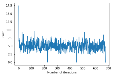
# visualising gradient descent
plt.plot(error_list)
plt.xlabel( "Number of iterations" )
plt.ylabel( "Cost" )
plt.show()输出如下:
偏差= [0.81830471]
系数= [[1.04586595]]
步骤#3:最后, 我们在测试集上进行预测并计算预测中的平均绝对误差。
# predicting output for X_test
y_pred = hypothesis(X_test, theta)
plt.scatter(X_test[:, 1 ], y_test[:, ], marker = '.' )
plt.plot(X_test[:, 1 ], y_pred, color = 'orange' )
plt.show()

# calculating error in predictions
error = np. sum (np. abs (y_test - y_pred) /y_test.shape[ 0 ])
print ( "Mean absolute error = " , error)
输出如下:
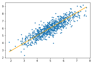
平均绝对误差= 0.4366644295854125
橙色线代表最终的假设函数:theta [0] + theta [1] * X_test [:, 1] + theta [2] * X_test [:, 2] = 0
首先, 你的面试准备可通过以下方式增强你的数据结构概念:Python DS课程。