ML算法：使用Sklearn实现OPTICS聚类

先决条件：OPTICS群集

本文将演示如何在Python中使用Sklearn实现OPTICS聚类技术。用于演示的数据集是商城客户细分数据可以从以下位置下载卡格勒.

步骤1：导入所需的库

import numpy as np
import pandas as pd
import matplotlib.pyplot as plt
from matplotlib import gridspec
from sklearn.cluster import OPTICS, cluster_optics_dbscan
from sklearn.preprocessing import normalize, StandardScaler

步骤2：载入资料

# Changing the working location to the location of the data
cd C:\Users\Dev\Desktop\Kaggle\Customer Segmentation
  
X = pd.read_csv( 'Mall_Customers.csv' )
  
# Dropping irrelevant columns
drop_features = [ 'CustomerID' , 'Gender' ]
X = X.drop(drop_features, axis = 1 )
  
# Handling the missing values if any
X.fillna(method = 'ffill' , inplace = True )
  
X.head()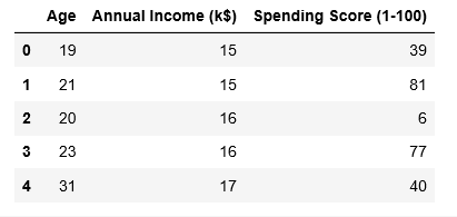

步骤3：预处理数据

# Scaling the data to bring all the attributes to a comparable level
scaler = StandardScaler()
X_scaled = scaler.fit_transform(X)
  
# Normalizing the data so that the data
# approximately follows a Gaussian distribution
X_normalized = normalize(X_scaled)
  
# Converting the numpy array into a pandas DataFrame
X_normalized = pd.DataFrame(X_normalized)
  
# Renaming the columns
X_normalized.columns = X.columns
  
X_normalized.head()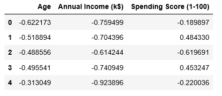

步骤4：构建聚类模型

# Building the OPTICS Clustering model
optics_model = OPTICS(min_samples = 10 , xi = 0.05 , min_cluster_size = 0.05 )
  
# Training the model
optics_model.fit(X_normalized)

步骤5：存储训练结果

# Producing the labels according to the DBSCAN technique with eps = 0.5
labels1 = cluster_optics_dbscan(reachability = optics_model.reachability_, core_distances = optics_model.core_distances_, ordering = optics_model.ordering_, eps = 0.5 )
  
# Producing the labels according to the DBSCAN technique with eps = 2.0
labels2 = cluster_optics_dbscan(reachability = optics_model.reachability_, core_distances = optics_model.core_distances_, ordering = optics_model.ordering_, eps = 2 )
  
# Creating a numpy array with numbers at equal spaces till
# the specified range
space = np.arange( len (X_normalized))
  
# Storing the reachability distance of each point
reachability = optics_model.reachability_[optics_model.ordering_]
  
# Storing the cluster labels of each point
labels = optics_model.labels_[optics_model.ordering_]
  
print (labels)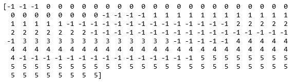

步骤6：可视化结果

# Defining the framework of the visualization
plt.figure(figsize = ( 10 , 7 ))
G = gridspec.GridSpec( 2 , 3 )
ax1 = plt.subplot(G[ 0 , :])
ax2 = plt.subplot(G[ 1 , 0 ])
ax3 = plt.subplot(G[ 1 , 1 ])
ax4 = plt.subplot(G[ 1 , 2 ])
  
# Plotting the Reachability-Distance Plot
colors = [ 'c.' , 'b.' , 'r.' , 'y.' , 'g.' ]
for Class, colour in zip ( range ( 0 , 5 ), colors):
     Xk = space[labels = = Class]
     Rk = reachability[labels = = Class]
     ax1.plot(Xk, Rk, colour, alpha = 0.3 )
ax1.plot(space[labels = = - 1 ], reachability[labels = = - 1 ], 'k.' , alpha = 0.3 )
ax1.plot(space, np.full_like(space, 2. , dtype = float ), 'k-' , alpha = 0.5 )
ax1.plot(space, np.full_like(space, 0.5 , dtype = float ), 'k-.' , alpha = 0.5 )
ax1.set_ylabel( 'Reachability Distance' )
ax1.set_title( 'Reachability Plot' )
  
# Plotting the OPTICS Clustering
colors = [ 'c.' , 'b.' , 'r.' , 'y.' , 'g.' ]
for Class, colour in zip ( range ( 0 , 5 ), colors):
     Xk = X_normalized[optics_model.labels_ = = Class]
     ax2.plot(Xk.iloc[:, 0 ], Xk.iloc[:, 1 ], colour, alpha = 0.3 )
      
ax2.plot(X_normalized.iloc[optics_model.labels_ = = - 1 , 0 ], X_normalized.iloc[optics_model.labels_ = = - 1 , 1 ], 'k+' , alpha = 0.1 )
ax2.set_title( 'OPTICS Clustering' )
  
# Plotting the DBSCAN Clustering with eps = 0.5
colors = [ 'c' , 'b' , 'r' , 'y' , 'g' , 'greenyellow' ]
for Class, colour in zip ( range ( 0 , 6 ), colors):
     Xk = X_normalized[labels1 = = Class]
     ax3.plot(Xk.iloc[:, 0 ], Xk.iloc[:, 1 ], colour, alpha = 0.3 , marker = '.' )
        
ax3.plot(X_normalized.iloc[labels1 = = - 1 , 0 ], X_normalized.iloc[labels1 = = - 1 , 1 ], 'k+' , alpha = 0.1 )
ax3.set_title( 'DBSCAN clustering with eps = 0.5' )
  
# Plotting the DBSCAN Clustering with eps = 2.0
colors = [ 'c.' , 'y.' , 'm.' , 'g.' ]
for Class, colour in zip ( range ( 0 , 4 ), colors):
     Xk = X_normalized.iloc[labels2 = = Class]
     ax4.plot(Xk.iloc[:, 0 ], Xk.iloc[:, 1 ], colour, alpha = 0.3 )
          
ax4.plot(X_normalized.iloc[labels2 = = - 1 , 0 ], X_normalized.iloc[labels2 = = - 1 , 1 ], 'k+' , alpha = 0.1 )
ax4.set_title( 'DBSCAN Clustering with eps = 2.0' )
  
  
plt.tight_layout()
plt.show()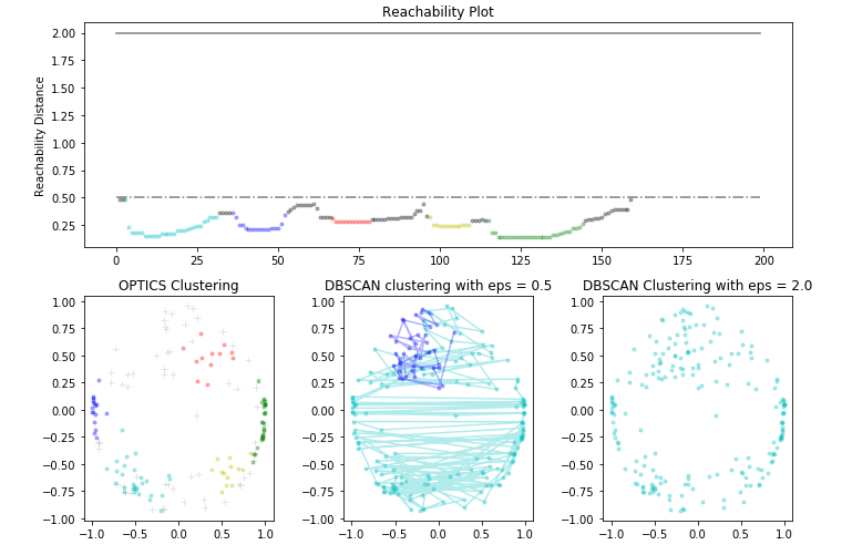

首先, 你的面试准备可通过以下方式增强你的数据结构概念：Python DS课程。

---