先决条件: K均值聚类
光谱聚类是一种不断发展的聚类算法, 在许多情况下, 其性能都优于许多传统的聚类算法。它将每个数据点视为一个图节点, 从而将聚类问题转换为图分区问题。一个典型的实现包括三个基本步骤:
建立相似度图:
此步骤以A表示的邻接矩阵的形式构建相似度图。可以按照以下方式构建邻接矩阵:-
- Epsilon邻域图:预先固定了参数ε。然后, 每个点都将连接到其epsilon半径中的所有点。如果任意两个点之间的所有距离的比例都相似, 则通常不存储边缘的权重, 即两个点之间的距离, 因为它们不提供任何其他信息。因此, 在这种情况下, 构建的图是无向且未加权的图。
- K最近邻居参数k是预先固定的。然后, 对于u和v的两个顶点, 只有当v在u的k个近邻中时, 才将边从u指向v。请注意, 这导致形成加权有向图, 因为并不总是这样, 对于每个具有v的u作为k个近邻中的一个, 对于v具有u的k个近邻中的情况将是相同的情况邻居。若要使该图无向, 请采用以下方法之一:
- 如果任一v在u的k个近邻中, 则将u的边从u定向到v, 并从v引导到uORu是v的k个近邻之一。
- 如果v位于u的k个近邻中, 则将边从u定向到v, 并从v定向到u和u是v的k个近邻之一。
- 完全连接图:为了构建此图, 每个点都连接有一个无向边权重, 该权重由两点到其他点之间的距离加权。由于此方法用于对局部邻域关系进行建模, 因此通常将高斯相似性度量用于计算距离。
将数据投影到较低的维度空间:
进行此步骤是为了考虑到同一簇的成员在给定维空间中可能相距很远的可能性。因此, 减少了维数空间, 从而使这些点在降维空间中更接近, 因此可以通过传统的聚类算法将它们聚类在一起。通过计算
图拉普拉斯矩阵
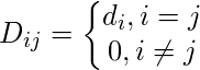
。首先要进行计算, 需要定义节点的程度。第i个节点的度为

注意

是上面邻接矩阵中定义的节点i和j之间的边缘。
度矩阵定义如下:
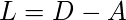
因此, 图拉普拉斯矩阵定义为:
然后将该矩阵归一化以提高数学效率。为了减小尺寸, 首先, 计算特征值和相应的特征向量。如果聚类的数量为k, 则采用第一特征值及其特征向量并将其堆叠到矩阵中, 从而使特征向量成为列。
集群数据:
此过程主要涉及通过使用任何传统的聚类技术(通常是K-Means聚类)对简化的数据进行聚类。首先, 为每个节点分配一行图拉普拉斯矩阵。然后, 使用任何传统技术对该数据进行聚类。为了转换聚类结果, 保留节点标识符。
特性:
- 假设少:与其他传统技术不同, 此聚类技术不假定数据遵循某些属性。因此, 这使该技术能够回答更为通用的聚类问题。
- 易于实施和速度:该算法比其他聚类算法更易于实现, 并且也非常快, 因为它主要由数学计算组成。
- 不可扩展:由于它涉及矩阵的构建以及特征值和特征向量的计算, 因此对于密集数据集而言非常耗时。
以下步骤演示了如何使用Sklearn实现光谱聚类。以下步骤的数据是信用卡资料可以从以下位置下载卡格勒.
步骤1:导入所需的库
import pandas as pd
import matplotlib.pyplot as plt
from sklearn.cluster import SpectralClustering
from sklearn.preprocessing import StandardScaler, normalize
from sklearn.decomposition import PCA
from sklearn.metrics import silhouette_score
步骤2:加载和清理数据
# Changing the working location to the location of the data
cd "C:\Users\Dev\Desktop\Kaggle\Credit_Card"

# Loading the data
X = pd.read_csv( 'CC_GENERAL.csv' )

# Dropping the CUST_ID column from the data
X = X.drop( 'CUST_ID' , axis = 1 )

# Handling the missing values if any
X.fillna(method = 'ffill' , inplace = True )

X.head()
步骤3:预处理数据以使数据可视化
# Preprocessing the data to make it visualizable

# Scaling the Data
scaler = StandardScaler()
X_scaled = scaler.fit_transform(X)

# Normalizing the Data
X_normalized = normalize(X_scaled)

# Converting the numpy array into a pandas DataFrame
X_normalized = pd.DataFrame(X_normalized)

# Reducing the dimensions of the data
pca = PCA(n_components = 2 )
X_principal = pca.fit_transform(X_normalized)
X_principal = pd.DataFrame(X_principal)
X_principal.columns = [ 'P1' , 'P2' ]

X_principal.head()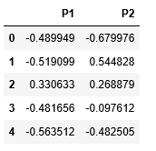
步骤4:构建聚类模型并可视化聚类
在以下步骤中, 将为参数"亲和力"使用两个具有不同值的光谱聚类模型。你可以阅读有关"光谱聚类"类的文档这里.
a)亲和力=" rbf"
# Building the clustering model
spectral_model_rbf = SpectralClustering(n_clusters = 2 , affinity = 'rbf' )

# Training the model and Storing the predicted cluster labels
labels_rbf = spectral_model_rbf.fit_predict(X_principal)
# Building the label to colour mapping
colours = {}
colours[ 0 ] = 'b'
colours[ 1 ] = 'y'
# Building the colour vector for each data point
cvec = [colours[label] for label in labels_rbf]
# Plotting the clustered scatter plot
b = plt.scatter(X_principal[ 'P1' ], X_principal[ 'P2' ], color = 'b' );
y = plt.scatter(X_principal[ 'P1' ], X_principal[ 'P2' ], color = 'y' );
plt.figure(figsize = ( 9 , 9 ))
plt.scatter(X_principal[ 'P1' ], X_principal[ 'P2' ], c = cvec)
plt.legend((b, y), ( 'Label 0' , 'Label 1' ))
plt.show()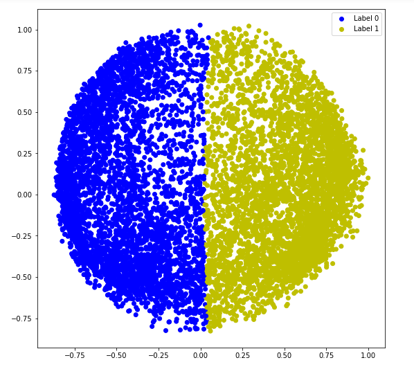
b)亲和力=" nearest_neighbors"
# Building the clustering model
spectral_model_nn = SpectralClustering(n_clusters = 2 , affinity = 'nearest_neighbors' )

# Training the model and Storing the predicted cluster labels
labels_nn = spectral_model_nn.fit_predict(X_principal)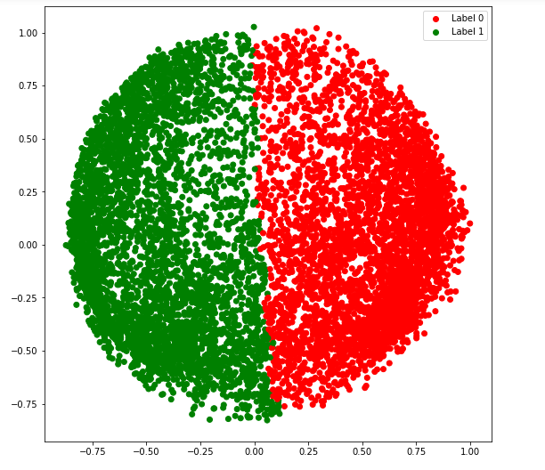
步骤5:评估成效
# List of different values of affinity
affinity = [ 'rbf' , 'nearest-neighbours' ]

# List of Silhouette Scores
s_scores = []

# Evaluating the performance
s_scores.append(silhouette_score(X, labels_rbf))
s_scores.append(silhouette_score(X, labels_nn))

print (s_scores)
步骤6:比较表演
# Plotting a Bar Graph to compare the models
plt.bar(affinity, s_scores)
plt.xlabel( 'Affinity' )
plt.ylabel( 'Silhouette Score' )
plt.title( 'Comparison of different Clustering Models' )
plt.show()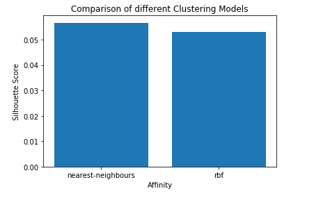
首先, 你的面试准备可通过以下方式增强你的数据结构概念:Python DS课程。